This document loads in some raw data, performs some filtering, and presents a plot and table of descriptive statistics. It then outputs the resulting file to be used in later analysis. Everything is contained within a single folder/R Project, and nested folders are used to keep the data organised.
The structure of this directory is like this. Using nested folders this way allows us to keep scripts, data, figures, and tables organised, rather than having everything sitting in one single folder.
We only need the tidyverse library for this analysis. The code cell below loads the library.
Code
library(tidyverse)
── Attaching core tidyverse packages ──────────────────────── tidyverse 2.0.0 ──
✔ dplyr     1.1.4     ✔ readr     2.1.5
✔ forcats   1.0.0     ✔ stringr   1.5.1
✔ ggplot2   3.5.1     ✔ tibble    3.2.1
✔ lubridate 1.9.3     ✔ tidyr     1.3.1
✔ purrr     1.0.2
── Conflicts ────────────────────────────────────────── tidyverse_conflicts() ──
✖ dplyr::filter() masks stats::filter()
✖ dplyr::lag()    masks stats::lag()
ℹ Use the conflicted package (<http://conflicted.r-lib.org/>) to force all conflicts to become errors
Data
The data is in the form of a .csv file, and is loaded in the same directory as this .qmd file. Since we are of course using an R Project or at least a .Rmd/.Qmd file, we do not have to worry about hard-coding our file paths, and can just type the name of the file. However, in order to go “into” the data folder, the filepath must include data/ before the filename.
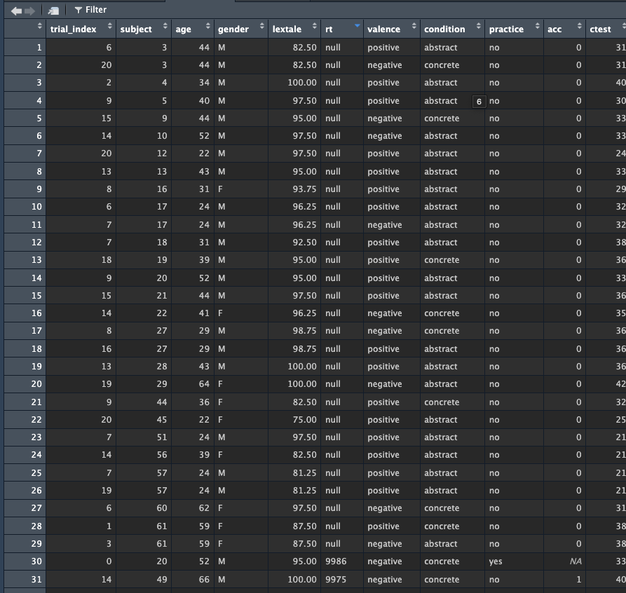
Load the data using the read_csv() function. Spend a moment to look at the column names and the structure of the data.
Code
raw_dat <-read_csv('data/raw_data.csv')
Rows: 1342 Columns: 11
── Column specification ────────────────────────────────────────────────────────
Delimiter: ","
chr (5): gender, rt, valence, condition, practice
dbl (6): trial_index, subject, age, lextale, acc, ctest

ℹ Use `spec()` to retrieve the full column specification for this data.
ℹ Specify the column types or set `show_col_types = FALSE` to quiet this message.
Clean the data
We see that there are some “practice” trials in these data, and we do not want to use these in our report. So we will filter these trials out from the data. Create a new variable, dat1, which is a copy of raw_data. Then, pipe into a filter() function which removes all rows where practice == 'yes'
Code
dat1 <- raw_dat %>%filter(practice =='no')
How many practice trials were removed?
Code
nrow(raw_dat) -nrow(dat1)
[1] 122
Fix the RT variable
Run a summary on the rt (reading time) variable. It is currently encoded as a character, but we need it to be a numerical value.
Code
summary(dat1$rt)
   Length     Class      Mode
     1220 character character
Why is it a character? because some answers are “null”!
Okay, let’s fix this by first removing all null values, and then transforming the variable using as.numeric(). Make a new variable, dat2, which is copy of dat1 and leads into a pipe which first filters out all rows where rt == null and then pipes into a mutate which transforms rt into numeric data.
   Min. 1st Qu.  Median    Mean 3rd Qu.    Max.
    774    5676    7904    8201   10556   18023
Plot the data
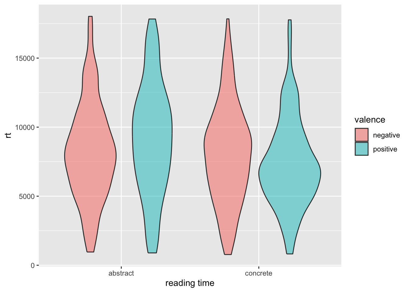
Let’s create a violin plot showing the RT data.
Code
ggplot(dat2, aes(y = rt, x = condition, fill = valence)) +geom_violin(alpha = .5, position ='dodge') +labs(x ="reading time", x ='')
Let’s pretend we like this figure - we can use ggsave() to save the figure to our folder, allowing us to use it in a presentation or word document or whatever. The function will automatically save the most recent rendered plot. Notice that I am saving the image to the figures/ folder! The function automatically chooses a size, which you can adjust by adding height and width arguments to the function.
Code
ggsave('figures/violin-plot.png', device ='png')
Saving 7 x 5 in image
Descriptive table
One way to quickly output a table of values is to create a dataframe and output is as a .csv file.
Let’s create summary statistics of rt in these conditions and then output the results. Recall we need to use group_by() and summarise() for this:
Now that we are done with our cleaning, plotting, and tables, let’s output the data for use in the next analysis. We will again use the write_csv() function, and give the data the name cleaned-data. We will put it into the data/ folder.
Code
write_csv(dat2, 'data/cleaned-data.csv')
The result is that you can now create a new.Rmd or .Qmd file which loads in cleaned-data.csv and operates on that data. You will not have to run everything in this notebook again. This compartmentalizes your analysis into stages and chunks which means you can work on it in discrete stages. Moreover, if you need to return to one part of the analysis, that is a matter of finding the right notebook for that particular step of the analysis. Of course, you can also render this file into html in order to provide your supervisors with a step-by-step look into what you’ve been doing!