About dprime
Dprime is a measure of sensitivity of responses to a given stimulus.
In a study such as Xin’s, there are four possible meanings behind any
valid response. We can adapt the Dprime sensitivity index from here
to match with Xin’s design:
Dprime(sensitivity index)
              ANSWERED YES    |  ANSWERED NO
 WORD    |     HIT            |  MISS
 NONWORD |     FALSE ALARM    |  CORRECT REJECTION
For Dprime, we care about two of these measures:
Hit Rate (H): proportion of WORD trials to which
subject responded YES = P("yes" | word) (the number of
times someone answered yes to a word trial / all word trials)
False Alarm rate (FA): proportion of NONWORD trials
to which subject responded YES = P("yes" | nonword) (the
number of times someone answered yes to a non-word trial / all non-word
trials)
Dprime (d’): Z(H)-Z(FA))
Dprime (d’) is caluclated using z-scores and uses the same logic as a
z-score, in that a z-score of 1 = one standard deviation from the
mean.
Typical d’ values are up to 2.0.
If a participant had 69% accuracy for both words and nonwords, their
d’ would be 1.0.
A value of d′ = 0 is chance (“guessing”) performance. interpreting dprime
Main tasks
- Calculate the counts for each item type
- Pivot wider
- Get rid of missing trials
- Calculate totals of word trials and non word trials
- Calculate the hit rate and false alarm rate
- Make the z scores using qnorm()
- Calculate dprime
- Plot dprime
library(tidyverse)
## ── Attaching packages ─────────────────────────── tidyverse 1.3.2 ──
## ✔ ggplot2 3.4.2     ✔ purrr   1.0.1
## ✔ tibble  3.2.1     ✔ dplyr   1.1.0
## ✔ tidyr   1.3.0     ✔ stringr 1.5.0
## ✔ readr   2.1.4     ✔ forcats 1.0.0
## ── Conflicts ────────────────────────────── tidyverse_conflicts() ──
## ✖ dplyr::filter() masks stats::filter()
## ✖ dplyr::lag()    masks stats::lag()
library(ggthemes)
Loading the dataset
You can download the dateset from here
or use read_csv() to import the data. The raw dataset can be saved as
‘df’.
df <- read_csv('https://stephenskalicky.com/r_data/dprime_data_raw.csv')
## Rows: 19711 Columns: 38
## ── Column specification ────────────────────────────────────────────
## Delimiter: ","
## chr (10): block, word, type, resp, vuw, condition, gender, test, otherL1, deci
## dbl (28): order, rt, list, cycle, sequence, age, score, year, LexTale, cscor...
##
## ℹ Use `spec()` to retrieve the full column specification for this data.
## ℹ Specify the column types or set `show_col_types = FALSE` to quiet this message.
There are loads of variables in the dataset but We will only need
three variables today: participant Id (vuw), wordtype (type) and
response (resp). Trim down the original dataset to only these variables
and save it as ‘df2’.
# tidyverse version
df2 <- df %>%
  dplyr::select(vuw, type, resp)

# base R version
df2 <- subset(df, select=c("vuw", "type", "resp"))
Inspect the “type” and “response” variables by converting them to a
factor (use levels(as.factor(x))). How does this data map
on to the sensitivity chart above?
levels(as.factor(df2$type))
## [1] "nonword" "word"
levels(as.factor(df2$resp))
## [1] "correct" "incorrect" "missing"
1. Calculate the counts for each item type
So we need a count of how many times each type of response was given
to both words and non-words.
Create a new df named scores from df2.
Calculate the raw counts of each type X response combination for each
participant.
You’ll need to use group_by(), summarise(),
and n().
# tidyverse version
scores.tv <- df2 %>%
  dplyr::group_by(vuw, type, resp) %>%
  dplyr::summarise(n = n())
## `summarise()` has grouped output by 'vuw', 'type'. You can override
## using the `.groups` argument.
# base R
scores.b <- as.data.frame(table(df2))
Your scores df should be like this:
glimpse(scores.tv)
## Rows: 302
## Columns: 4
## Groups: vuw, type [124]
## $ vuw  <chr> "009d3700", "009d3700", "009d3700", "009d3700", "009d3700", "009d…
## $ type <chr> "nonword", "nonword", "nonword", "word", "word", "word", "nonword…
## $ resp <chr> "correct", "incorrect", "missing", "correct", "incorrect", "missi…
## $ n    <int> 92, 65, 1, 151, 12, 1, 111, 47, 133, 29, 1, 103, 55, 152, 12, 83,…
2. Pivot the data wider
To better calculate the proportion of correct and incorrect answers
in word and nonword trials, let’s pivot the data into wide format and
save it as scores2. The key arguments are
names_from and values_from.
# tidyverse
scores2.tv <- scores.tv %>%
  pivot_wider(names_from = c(type, resp), values_from = n)


# base R (probably more efficient)
library(reshape2)
##
## Attaching package: 'reshape2'
## The following object is masked from 'package:tidyr':
##
##     smiths
scores2.b <- dcast(df2, vuw ~ type + resp)
## Using resp as value column: use value.var to override.
## Aggregation function missing: defaulting to length
3. Get rid of missing trials & 4. Calculate totals of word
trials and non word trials
Remember our formula for hit rate and false alarm rate?
HIT RATE = number of word-correct trials / total number of word
trials
FALSE ALARM = number of nonword-incorrect trials / total number of
non-word trials
So we don’t need the missing trials. We also need to
know the total number of word trials and non-word trials, per
participant.
Create a new df named scores3 from
scores2.
In a single pipe:
- remove the two columns associated with missing data - create a new
column named word_trials which is the sum of all real word
trials - create a ner column named nw_trials which is the
sum of all non-word trials
# tidyverse version
scores3.tv <- scores2.tv %>%
  dplyr::select(-word_missing, -nonword_missing) %>%
  dplyr::mutate(word_trials = word_correct + word_incorrect, nw_trials = nonword_correct + nonword_incorrect)

# base R version
scores3.b <- subset(scores2.b, select = c(-word_missing, -nonword_missing))

# add total trials
scores3.b$word_trials <- scores3.b$word_correct + scores3.b$word_incorrect
scores3.b$nw_trials <- scores3.b$nonword_correct + scores3.b$nonword_incorrect
5. Calculate the hit rate and false alarm rate
Now we can calculate the hit rate and false alarm rate. Create a new
df scores4 from scores3.
Create a new column hit_rate which is the proportion of
word-correct / all word trials.
Create a new column named false_alarm which is the
proportion of nonword-incorrect / all non-word trials.
# tidyverse version
scores4.tv <- scores3.tv %>%
  #dplyr::mutate(hit_rate = round(word_correct / word_trials*100, 2), false_alarm = nonword_incorrect / nw_trials*100)
  dplyr::mutate(hit_rate = word_correct / word_trials, false_alarm = nonword_incorrect / nw_trials)

# base R
scores4.b <- scores3.b

# guess base R is better
# a shortcut to not have to type x$ is to use with, then it makes it available.
scores4.b$hit_rate <- with(scores4.b, word_correct / word_trials)
scores4.b$false_alarm <- with(scores4.b, nonword_incorrect / nw_trials)
6. Make the z scores using qnorm() & 7. Calculate dprime
Now we should be able to caclulate our own d prime (d’).
We can use qnorm() to get z scores for our values
(because the z-scores actually come from the subtracted product and not
the values themselves - don’t worry about this too much - just use
qnorm() in your pipe to make the new values.).
Let’s create a df scores5 by adding another three
columns to scores4:
HRz for the qnorm() of hit rate
FAz for qnorm of false alarm rate dprime for dprime
(d' = Z(Hit rate)-Z(False alarm))
8. Plot dprime
Now we can plot the data! Before that, let’s create a df named
plot.data as we need hit rate, false alarm rate and dprime
only - so select only those columns (this isn’t necessary at all).
# tidyverse
plot.data.tv <- scores5.tv %>%
  ungroup() %>%
  dplyr::select(hit_rate, false_alarm, dprime)

# base R
plot.data.b <- subset(scores5.b, select = c(hit_rate, false_alarm, dprime))
Your ‘plot.data’ should look like this.
head(plot.data.tv)
## # A tibble: 6 × 3
##   hit_rate false_alarm dprime
##      <dbl>       <dbl>  <dbl>
## 1    0.926      0.414    1.67
## 2    0.821      0.297    1.45
## 3    0.927      0.348    1.84
## 4    0.877      0.471    1.23
## 5    0.758      0.149    1.74
## 6    0.938      0.0321   3.39
Time to visualize the data! Create a ggplot with hit rate on the y
axis and false alarm rate on the x axis.
Add a geom_text which takes dprime as the
label within the aes call. Also add
color = dprime outside the aes but within the
geom_text call.
Add theme_gdocs() to the end of your plot.
library(ggthemes)
ggplot(plot.data.b, aes(x = false_alarm, y = hit_rate, label = round(dprime, 2), color = dprime)) +
  geom_text() +
 # xlim(0,1) +
  #ylim(0,1) +
  coord_cartesian(xlim = c(0,1), ylim = c(0,1)) +
  geom_abline(slope = 1, alpha = .5, color = 'red', linetype = 2) +
  theme_gdocs()
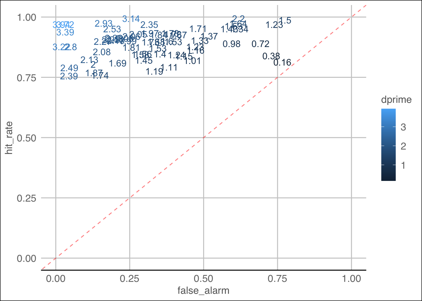
Key observations:
- Nature of data shows participants are, in general, pretty good at
the real word trials - hit rate is overall quite high
- Lots of participants grouped in top right corner which shows that
for the most part they are doing ok
- Four participants with a dprime < 1, one with near 0 (0.16).
However, can we truly know if this is a result of malicious
behaviour?
- Maybe cluster analysis could help? (shrug)
Conclusion - need to cross reference this to other data, such as RT,
longstring, and more.