zscores
Stephen Skalicky
08/09/2021
Zed scores and you
Consider a situation where you measure performance on two tests of lexical knowledge. One test is 25 items worth 2 points each with a total possible score of 0-50. The second test is 10 items, each worth up to 10 points, for a total possible score of 0-100.
Let’s first simulate this data for a hypothetical 100 participants.
Create two objects, test1_possible_scores and
test2_possible_scores. Using the seq function,
set the correct possible range for each test.
test1_possible_scoresrange is 0 to 50, iterating by 2test2_possible_scoresrange is 0 to 100, iterating by 10
test1_possible_scores <- seq(0,50,2)
test2_possible_scores <- seq(0,100,10)
test1_possible_scores
## [1] 0 2 4 6 8 10 12 14 16 18 20 22 24 26 28 30 32 34 36 38 40 42 44 46 48
## [26] 50test2_possible_scores## [1] 0 10 20 30 40 50 60 70 80 90 100You should see something like this:
 [1]  0  2  4  6  8 10 12 14 16 18 20 22 24 26 28 30 32 34 36 38 40 42 44 46 48 50
 [1]   0  10  20  30  40  50  60  70  80  90 100
Now use a set.seed with the value 092021 to
generate 100 samples from each test. Name your variables
test1sample and test2sample. Use the
sample() function, with the argument
replace = TRUE
set.seed(092021)
test1sample <- sample(test1_possible_scores, 100, replace = TRUE)
test2sample <- sample(test2_possible_scores, 100, replace = TRUE)
test1sample
## [1] 46 42 8 50 22 20 8 14 42 16 4 24 50 20 50 22 2 48 24 18 10 20 28 40 36
## [26] 12 0 48 6 46 44 44 22 24 2 34 48 26 14 28 46 40 48 18 42 4 6 38 18 40
## [51] 34 44 32 30 4 6 0 34 22 22 38 50 28 20 28 30 34 22 50 6 30 32 30 6 14
## [76] 10 46 26 50 0 16 4 2 30 14 46 24 50 28 42 36 16 44 6 10 36 0 0 40 30test2sample## [1] 60 20 50 30 90 20 70 70 70 60 10 20 30 90 100 90 50 30
## [19] 60 80 10 90 10 50 80 80 40 80 100 80 80 50 10 100 20 50
## [37] 70 90 30 70 80 20 20 0 80 60 70 0 10 90 100 50 90 0
## [55] 90 90 40 50 60 90 50 40 40 30 0 10 80 90 10 90 10 20
## [73] 50 100 30 50 60 10 10 80 100 100 20 70 0 40 90 10 50 90
## [91] 10 50 10 40 0 10 100 20 90 30You should get data that looks like this:
 test2sample
  [1] 46 42  8 50 22 20  8 14 42 16  4 24 50 20 50 22  2 48 24 18 10 20 28 40 36 12  0 48  6 46 44 44 22 24  2 34 48 26 14
 [40] 28 46 40 48 18 42  4  6 38 18 40 34 44 32 30  4  6  0 34 22 22 38 50 28 20 28 30 34 22 50  6 30 32 30  6 14 10 46 26
 [79] 50  0 16  4  2 30 14 46 24 50 28 42 36 16 44  6 10 36  0  0 40 30

 test2sample
  [1]  60  20  50  30  90  20  70  70  70  60  10  20  30  90 100  90  50  30  60  80  10  90  10  50  80  80  40  80 100
 [30]  80  80  50  10 100  20  50  70  90  30  70  80  20  20   0  80  60  70   0  10  90 100  50  90   0  90  90  40  50
 [59]  60  90  50  40  40  30   0  10  80  90  10  90  10  20  50 100  30  50  60  10  10  80 100 100  20  70   0  40  90
 [88]  10  50  90  10  50  10  40   0  10 100  20  90  30
Now create a tibble named zed01 with three
columns:
subject, which is the number range 1:100test1, which is the objecttest1sampletest2, which is the objecttest2sample
zed01 <- tibble(subject = 1:100,
                test1 = test1sample,
                test2 = test2sample)

str(zed01)
## tibble [100 × 3] (S3: tbl_df/tbl/data.frame)
## $ subject: int [1:100] 1 2 3 4 5 6 7 8 9 10 ...
## $ test1 : num [1:100] 46 42 8 50 22 20 8 14 42 16 ...
## $ test2 : num [1:100] 60 20 50 30 90 20 70 70 70 60 ...You should see something like this when running
str(zed01)
tibble [100 × 3] (S3: tbl_df/tbl/data.frame)
 $ subject: int [1:100] 1 2 3 4 5 6 7 8 9 10 ...
 $ test1  : num [1:100] 46 42 8 50 22 20 8 14 42 16 ...
 $ test2  : num [1:100] 60 20 50 30 90 20 70 70 70 60 ...
What is the mean and sd of our two test scores? We don’t need to be
fancy, you can just run mean() and sd() on the
two columns.
Mean and SD for zed01$test1
mean(zed01$test1)## [1] 26.14sd(zed01$test1)## [1] 15.72556Mean and SD for zed02$test2
mean(zed01$test2)## [1] 51.7sd(zed01$test2)## [1] 32.56865We might want to visualize the data in order to see the range of test
scores. Before we do that, let’s use pivot_longer to
combine our test scores into a single column, with the resulting columns
being named test and score. Create a new
tibble named zed02 from zed01 to do this.
pivot_longer(cols = c(), names_to = '', values_to = '')
zed02 <- zed01 %>%
  pivot_longer(cols = c(test1, test2), names_to = 'test', values_to = 'score')
Create a ggplot from zed02, with test on the y-axis and
score on the x-axis. Add a geom_boxplot geom
to your plot. Then add a geom_jitter() with
alpha = .5.
What do you see?
ggplot(zed02, aes(x= score, y = test)) +
  geom_boxplot() +
  geom_jitter(alpha = .5)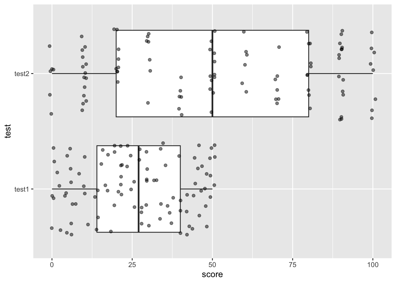
The issue is that we can’t meaningfully compare these scores because they are on different scales. The solution to this is to use z-scores, which standardize any set of values to be on the same scale. To calculate a z score, use this formula
For each value:

(value - mean)/sd
Since we already know how to calculate mean and sd, we should be able to do this pretty easily. Let’s use zed01 to create z-score versions of our variables.
Create a new tibble named zed03 fromzed01.
Using mutate, create two new columns which are the z-scores
of test1 and test2. Name them
test1z and test2z. Use the formula above (and
not any pre-existing functions). You need to be very
careful how you place your brackets so that order of operations is
applied correctly.
# Put your code here
zed03 <- zed01 %>%
      mutate(test1z = (test1 - mean(test1))/sd(test1),
             test2z = (test2 - mean(test2))/sd(test2))
If successful you should see this when running
str(zed03)
tibble [100 × 5] (S3: tbl_df/tbl/data.frame)
 $ subject: int [1:100] 1 2 3 4 5 6 7 8 9 10 ...
 $ test1  : num [1:100] 46 42 8 50 22 20 8 14 42 16 ...
 $ test2  : num [1:100] 60 20 50 30 90 20 70 70 70 60 ...
 $ test1z : num [1:100] 1.263 1.009 -1.154 1.517 -0.263 ...
 $ text2z : num [1:100] 0.2548 -0.9733 -0.0522 -0.6663 1.176 ...
Make a new tibble named zed04 from zed03.
Then use pivot_longer on your regular and z-scored
variables to create new columns with the same names you used for
zed02 (test and score).
zed04 <- zed03 %>%
  pivot_longer(cols = c(test1, test2, test1z, test2z), names_to = 'test', values_to = 'score')
str(zed04)
## tibble [400 × 3] (S3: tbl_df/tbl/data.frame)
## $ subject: int [1:400] 1 1 1 1 2 2 2 2 3 3 ...
## $ test : chr [1:400] "test1" "test2" "test1z" "test2z" ...
## $ score : num [1:400] 46 60 1.263 0.255 42 ...Make a new tibble named zed04z which includes
subject and the z-scored values using
filter(). We want to filter so that ONLY test1z and ONLY
test2z remain in the data.
zed04z <- zed04 %>%
 # filter(str_detect(test, 'z'))
  filter(test == 'test1z' | test == 'test2z')

str(zed04z)
## tibble [200 × 3] (S3: tbl_df/tbl/data.frame)
## $ subject: int [1:200] 1 1 2 2 3 3 4 4 5 5 ...
## $ test : chr [1:200] "test1z" "test2z" "test1z" "test2z" ...
## $ score : num [1:200] 1.263 0.255 1.009 -0.973 -1.154 ...Recreate the same ggplot as you did before. What do you see now?
ggplot(zed04z, aes(y = test, x = score )) +
  geom_boxplot() +
  geom_jitter(alpha = .5)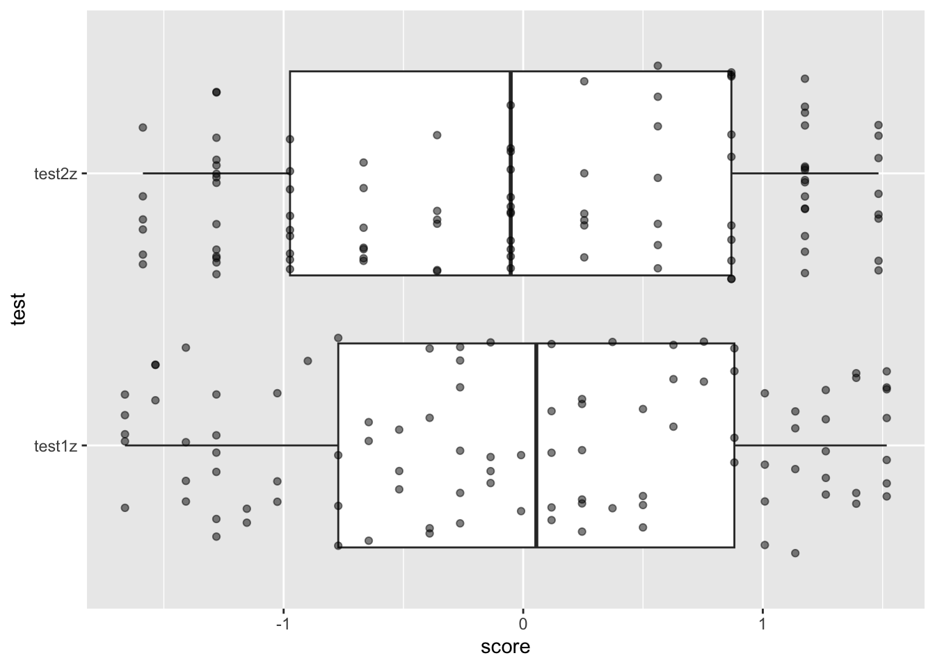
When you z-score a variable, you set the mean = to 0, with each increase in one unit = 1 standard deviation. This is incredibly useful when modelling and visualizing data (and in fact basically a requirement for regression.)
To demonstrate this, let’s create a final plot which includes our raw
and z-score variables side by side. Create a ggplot from
zed04 which uses the same boxplot and jitter as the
previous plot. However, before those commands, use a
facet_wrap(. ~ test, scales = 'free')
ggplot(zed04, aes(y = test, x = score)) +
  facet_wrap(. ~ test, scales = 'free') +
  geom_boxplot() +
  geom_jitter(alpha = .5, width = .1)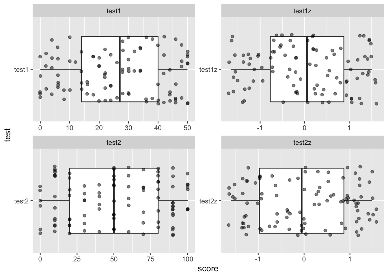
You should notice that we actually haven’t “changed” the data fundamentally, instead we have “transformed” it by applying the same transformation to all data points.
If you want to get fancy you can play with other packages, like
ggridges to get different types of visualizations. Replace
the boxplot and jitter with a geom_density_ridge() to get
the following plot (you’ll need to
install.packages(ggridges))
install.packages('ggridge')
library(ggridges)

ggplot(zed04z, aes(x = score, y = test)) +
  geom_density_ridges(aes(fill = test), alpha = .5)
## Picking joint bandwidth of 0.358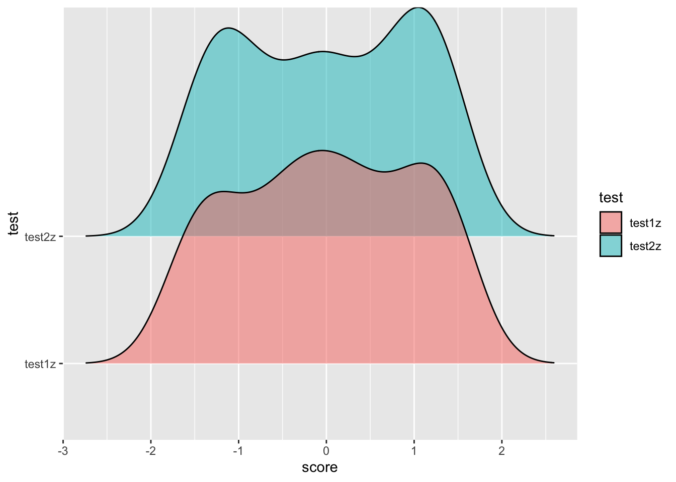
And, by the way, you can just use scale() to z-score
things automatically without having to use the formula. Here is an
example below that will apply a mutate across all columns, and then use
as.vector() to strip the attributes associated with the
transformation.
zed05 <- zed01 %>%
  mutate(across(.cols = c(test1, test2), scale, center = T, scale = T)) %>%
  mutate(across(everything(), as.vector))
## Warning: There was 1 warning in `mutate()`.
## ℹ In argument: `across(.cols = c(test1, test2), scale, center = T,
## scale = T)`.
## Caused by warning:
## ! The `...` argument of `across()` is deprecated as of dplyr 1.1.0.
## Supply arguments directly to `.fns` through an anonymous function
## instead.
##
## # Previously
## across(a:b, mean, na.rm = TRUE)
##
## # Now
## across(a:b, \(x) mean(x, na.rm = TRUE))