data cleaning - vocab size

Thanks to TJ for providing the data and guiding us through the discussion!

The goal of this lesson is to practice data wrangling and exploration with less scaffolding. TJ has provided a data set and what that final data set should look like.

Loading and observing the dataset

More often than not, raw data looks very different to data that appears in a publication. This means that a lot of time is spent cleaning the data. In this exercise, we will practice the process of cleaning up data. The first thing we need to do is import the data and look at it.

You can download the data from here.

Or you can pass the URL directly to read_csv to get the data into R.

dat <- read_csv('https://www.stephenskalicky.com/r_data/testData.csv')

## Rows: 19 Columns: 109
## ── Column specification ────────────────────────────────────────────
## Delimiter: ","
## dbl (109): ID, Age, vlt.2k, vlt.3k, vlt.5k, vlt.10k, vlt.aca, test.vst, orde...
## 
## ℹ Use `spec()` to retrieve the full column specification for this data.
## ℹ Specify the column types or set `show_col_types = FALSE` to quiet this message.

Examine the data. What does each row represent? What are the column names?

Main task

What is the score for each participant, and what is their vocabulary size?

In order to answer these questions we need to do a variety of things.

In the session, we decided it would be fun to compare and contrast the tidyverse and base r methods to answer these questions. The objects with tv at the end are the tidyverse methods, while the objects with b at the end are base R.

the first task is to get only the VST data (don’t need anything related to levels, age, etc.).

# subset VST data (so we want ID + all of the columns with vst.qX in the name)

# pipe using tidyverse
vst_data_tv <- dat %>%
  dplyr::select(c(ID, contains('vst.')))

# subset function from base R
vst_data_b <- subset(dat, select = grep("ID|vst.", names(dat), value = T))

identical(vst_data_tv, vst_data_b)

## [1] TRUE

the next task is to remove anyone who has NA for a vst test

# remove NAs (n should = 16) (any row that has an NA anywhere)

# Tidyverse will drop a row where ANY column has an NA
vst_data_tv1 <- vst_data_tv %>%
  drop_na(vst.q1)

# Slicing with Base R - looking for NA in the second column only
# Slicing is a technique used by other programming language (with different syntax) - so it can be a useful method but harder to read
vst_data_b1 <- vst_data_b[!is.na(vst_data_b[,2]),]

in case you want to go through some potentially redundant steps here they are

compute sums for each ten questions that make up a 1k freq band rename datvst_summed_by_level's columns to appropriate names

the next step is to create a table/df/tibble with three columns: person, total score (VST), and total vocabulary (Vsize)

# create a table of person, total score, total vocab size
# the vst ranges from 0 - 100. let's calculate each subject's score on the vst.


# tidyverse method one
vst_data_tv2 <- vst_data_tv1 %>%
  rowwise(ID) %>% 
  mutate(VST = sum(c_across(contains('vst'))))

# tidyverse method two (via Micky Vale)
vst_data_tv2 <- vst_data_tv1 %>%
    mutate(VST = rowSums(select(., contains('vst'))))

# glue it into a df. 
finalResults_tv <- tibble(person = vst_data_tv1$ID, VST = vst_data_tv2$VST)
  
# baseRisbestR
# will need to use apply here because this needs to be done row-wise (i think?)
vst_data_b2 <- apply(vst_data_b1[,2:ncol(vst_data_b1)], 1, sum)

finalResults_b <- data.frame(person = vst_data_b1$ID, VST = vst_data_b2)


finalResults_b <- data.frame(person = vst_data_b1$ID, VST = vst_data_b2, Vsize = vst_data_b2*200)

finalResults2 <- vst_data_tv1 %>%
     mutate(person = ID, VST = rowSums (select(., contains ('vst'))), Vsize = VST * 200) %>%
     select(person, VST, Vsize)

add Vsize (this is also done above - we adjusted the above code after doing the below). This shows you that Vsize was just VST*200.

# add one more column which is vsize
# what is vsize? Well, it looks like each correct answer is indicative of 200 words or something like that
# so we can easily create a new column by multiplying VST*200

# we can actually use mutate here...
finalResults_tv <- finalResults_tv %>%
  mutate(Vsize = VST * 200)

# what about base R? 
finalResults_b['Vsize'] <- finalResults_b$VST*200
# this is probably a better way to to do it this way
finalResults_b$Vsize <- finalResults_b[,'VST'] * 200

plots for fun

ggplot(finalResults_b, aes(x = VST, y = Vsize)) +
  #geom_point() + 
  geom_text(aes(label = person))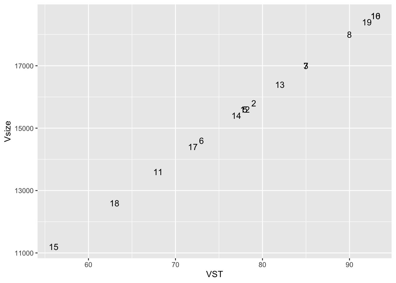

Your final dataframe should look like this:

person  VST     Vsize
01         79     15800
02         85     17000
03         78     15600
04         73     14600
05         85     17000
06         90     18000
07         93     18600
08         68     13600
09         78     15600
10         82     16400
11         77     15400
12         56     11200
13         93     18600
14         72     14400
15         63     12600
16         92     18400