#install.packages('tidyverse')Chapter 2
Sections 2.1 to 2.6
2.1 Introduction
“This chapter is very technical. If you feel overwhelmed, don’t worry” (Winter, 2020, p. 27).
Install ‘tidyverse’ if you haven’t already done so.
Load all the packages that we will be using.
library(tidyverse)── Attaching core tidyverse packages ──────────────────────── tidyverse 2.0.0 ──
✔ dplyr 1.1.4 ✔ readr 2.1.5
✔ forcats 1.0.1 ✔ stringr 1.5.2
✔ ggplot2 4.0.0 ✔ tibble 3.3.0
✔ lubridate 1.9.4 ✔ tidyr 1.3.1
✔ purrr 1.1.0
── Conflicts ────────────────────────────────────────── tidyverse_conflicts() ──
✖ dplyr::filter() masks stats::filter()
✖ dplyr::lag() masks stats::lag()
ℹ Use the conflicted package (<http://conflicted.r-lib.org/>) to force all conflicts to become errorslibrary(tibble)
library(readr)
library(dplyr)
library(magrittr)
Attaching package: 'magrittr'

The following object is masked from 'package:purrr':

    set_names

The following object is masked from 'package:tidyr':

extractlibrary(ggplot2)===============================================================================================================
2.2 tibble and readr
Let’s load some data with read.csv () and convert the data frame to tibble.
# Load data
AmE_demo <- read.csv("AmE_demo.csv")

# Convert to tibble
AmE_demo <- as_tibble(AmE_demo)
AmE_demo
# A tibble: 202 × 10
Duration ResponseId Age Gender Education L1 Country.of.birth
<int> <chr> <int> <chr> <chr> <chr> <chr>
1 704 R_1aDoqaqxlpUIkiy 28 Female Undergraduate Engl… USA
2 751 R_8BbNFuwLGNEK2Qv 27 female undergraduate engl… united states
3 958 R_5YmJvQir3sng7yP 20 Male Some college … Engl… United States o…
4 1562 R_4jGPhlwWcfhMdcJ 60 female undergraduate… Engl… United States
5 1011 R_1CJjszbl83LOWUy 38 Female Postgraduate Engl… New Jersey
6 1072 R_2j1YU3bmjLfu1Oa 65 female Master's Degr… Engl… Hershey, PA
7 1159 R_46gLJtNh32Ybrf7 30 Female Associate's D… Engl… America
8 509 R_7CTqax3AWEpEqnn 29 female undergraduate engl… new york
9 1757 R_1egBkgJmbWMtp1P 33 Female bachelor's de… Engl… Alabama, United…
10 1229 R_1qwaXrXju6PWsCg 56 Male Masters degree Engl… Vietnam
# ℹ 192 more rows
# ℹ 3 more variables: Country.of.residence <chr>, Foreign.countries <chr>,
# Foreign.countries_2_TEXT <chr># < > = vector classes
# chr = character, int = integer, fct = factor, dbl = double
# Note that Bbase R function read.csv() automatically interprets any text column as factor, so although tibbles default to character vectors, before the df was converted a character-to-factor conversion has already happened (Winer, 2020, p.29). So we can use read_csv() to avoid this.
# (This did not happen here though and I didn't want to try make it happen...)
# Duration = time used to complete the surveyLet’s load some data with read_csv () which runs faster than read.csv() and also creates tibbles by default yay :)
# Load data
AmE_demo <- read_csv("AmE_demo.csv")
Rows: 202 Columns: 10
── Column specification ────────────────────────────────────────────────────────
Delimiter: ","
chr (8): ResponseId, Gender, Education, L1, Country.of.birth, Country.of.res...
dbl (2): Duration, Age
ℹ Use `spec()` to retrieve the full column specification for this data.
ℹ Specify the column types or set `show_col_types = FALSE` to quiet this message.AmE_demo# A tibble: 202 × 10
Duration ResponseId Age Gender Education L1 Country.of.birth
<dbl> <chr> <dbl> <chr> <chr> <chr> <chr>
1 704 R_1aDoqaqxlpUIkiy 28 Female Undergraduate Engl… USA
2 751 R_8BbNFuwLGNEK2Qv 27 female undergraduate engl… united states
3 958 R_5YmJvQir3sng7yP 20 Male Some college … Engl… United States o…
4 1562 R_4jGPhlwWcfhMdcJ 60 female undergraduate… Engl… United States
5 1011 R_1CJjszbl83LOWUy 38 Female Postgraduate Engl… New Jersey
6 1072 R_2j1YU3bmjLfu1Oa 65 female Master's Degr… Engl… Hershey, PA
7 1159 R_46gLJtNh32Ybrf7 30 Female Associate's D… Engl… America
8 509 R_7CTqax3AWEpEqnn 29 female undergraduate engl… new york
9 1757 R_1egBkgJmbWMtp1P 33 Female bachelor's de… Engl… Alabama, United…
10 1229 R_1qwaXrXju6PWsCg 56 Male Masters degree Engl… Vietnam
# ℹ 192 more rows
# ℹ 3 more variables: Country.of.residence <chr>, Foreign.countries <chr>,
# Foreign.countries_2_TEXT <chr>Winter also mentioned another function read_delim() which reads files that are not csv. But well, just save your data in csv I guess.
# x <- read_delim('example_file.txt', delim = '\t')
# "delim =" specifies what character separates the columns.Here is tab '\t'.
===============================================================================================================
2.3 dplyr
“The dplyr package (Wickham et al., 2018) is the tidyverse’s workhorse for changing
tibbles” (Winter, p. 30). This section goes through some functions that helps organize our tibbles/data.
For example, we can use filter() to reduce the demo tibble to only those with age over 40:
filter(AmE_demo, Age > 40)# A tibble: 73 × 10
Duration ResponseId Age Gender Education L1 Country.of.birth
<dbl> <chr> <dbl> <chr> <chr> <chr> <chr>
1 1562 R_4jGPhlwWcfhMdcJ 60 female undergraduate… Engl… United States
2 1072 R_2j1YU3bmjLfu1Oa 65 female Master's Degr… Engl… Hershey, PA
3 1229 R_1qwaXrXju6PWsCg 56 Male Masters degree Engl… Vietnam
4 1467 R_2bOaZP0hEQucH1Q 42 Female Bachelor’s Engl… New Jersey
5 1258 R_5MS3ovmRuVSOWyK 65 female undergraduate Engl… California, USA
6 678 R_1eh8DBv0fWjH1yf 43 male undergrad engl… California, usa
7 1145 R_1b2ynWgb9oqcdAC 62 Female AA degree Engl… America
8 1135 R_2NhlnREre6wsaWI 42 male some college engl… Atlanta, GA
9 2236 R_6smK5LjW6XivQHJ 50 female postgraduate engl… United States
10 1431 R_6Teo5SMTpSAtM5P 45 Female Associates de… Engl… 1978
# ℹ 63 more rows
# ℹ 3 more variables: Country.of.residence <chr>, Foreign.countries <chr>,
# Foreign.countries_2_TEXT <chr>Or we can look at the data for those who have lived in foreign countries:
filter(AmE_demo, Foreign.countries == "Yes")# A tibble: 35 × 10
Duration ResponseId Age Gender Education L1 Country.of.birth
<dbl> <chr> <dbl> <chr> <chr> <chr> <chr>
1 704 R_1aDoqaqxlpUIkiy 28 Female Undergraduate Engl… USA
2 1072 R_2j1YU3bmjLfu1Oa 65 female Master's Degr… Engl… Hershey, PA
3 1757 R_1egBkgJmbWMtp1P 33 Female bachelor's de… Engl… Alabama, United…
4 1229 R_1qwaXrXju6PWsCg 56 Male Masters degree Engl… Vietnam
5 822 R_2Kd9xBx8hxMmPOK 25 female undergradute engl… united states
6 781 R_1r9xS6EAQPp6JlU 32 female masters degree engl… USA
7 1605 R_2Cl7kEPO0iEGNTk 53 female some college engl… 1970
8 2318 R_6KBqiUc3A1ySR3z 30 Female MSc (Masters) Engl… United Kingdom
9 1231 R_1QfIXR7E5orbvem 43 Female Master's of A… Engl… 1980
10 2930 R_1jCdpFyYS3xhgfJ 35 Female 4 year colleg… Engl… Nigeria
# ℹ 25 more rows
# ℹ 3 more variables: Country.of.residence <chr>, Foreign.countries <chr>,
# Foreign.countries_2_TEXT <chr>filter() restricts the data to a subset of rows, so basically it filters rows. When we want to select particular columns, we can select():
select(AmE_demo, Age, Gender, Education)# A tibble: 202 × 3
Age Gender Education
<dbl> <chr> <chr>
1 28 Female Undergraduate
2 27 female undergraduate
3 20 Male Some college but no degree
4 60 female undergraduate degree - BFA
5 38 Female Postgraduate
6 65 female Master's Degree
7 30 Female Associate's Degree
8 29 female undergraduate
9 33 Female bachelor's degree
10 56 Male Masters degree
# ℹ 192 more rowsWe can also use the minus sign to exclude a column:
select(AmE_demo, -ResponseId)# A tibble: 202 × 9
Duration Age Gender Education L1 Country.of.birth Country.of.residence
<dbl> <dbl> <chr> <chr> <chr> <chr> <chr>
1 704 28 Female Undergradu… Engl… USA Philadelphia
2 751 27 female undergradu… engl… united states helena
3 958 20 Male Some colle… Engl… United States o… San Diego
4 1562 60 female undergradu… Engl… United States New Orleans suburb
5 1011 38 Female Postgradua… Engl… New Jersey Howell
6 1072 65 female Master's D… Engl… Hershey, PA Newville, PA
7 1159 30 Female Associate'… Engl… America Grand Rapids
8 509 29 female undergradu… engl… new york Brooklyn
9 1757 33 Female bachelor's… Engl… Alabama, United… Ellenwood, GA
10 1229 56 Male Masters de… Engl… Vietnam Champaign, IL
# ℹ 192 more rows
# ℹ 2 more variables: Foreign.countries <chr>, Foreign.countries_2_TEXT <chr>We can also use colon to select consecutive columns:
select(AmE_demo, L1:Foreign.countries)# A tibble: 202 × 4
L1 Country.of.birth Country.of.residence Foreign.countries
<chr> <chr> <chr> <chr>
1 English USA Philadelphia Yes
2 english united states helena No
3 English United States of America San Diego No
4 English United States New Orleans suburb No
5 English New Jersey Howell No
6 English Hershey, PA Newville, PA Yes
7 English America Grand Rapids No
8 english new york Brooklyn No
9 English Alabama, United States Ellenwood, GA Yes
10 English Vietnam Champaign, IL Yes
# ℹ 192 more rowsNow since we do not like capiticalised column names nor column names with full stops, we can rename them:
AmE_demo <- rename(AmE_demo, duration = Duration, id = ResponseId, age = Age, gender = Gender, ed = Education, birthplace = Country.of.birth, residence = Country.of.residence, abroad = Foreign.countries, where = Foreign.countries_2_TEXT)

AmE_demo
# A tibble: 202 × 10
duration id age gender ed L1 birthplace residence abroad where
<dbl> <chr> <dbl> <chr> <chr> <chr> <chr> <chr> <chr> <chr>
1 704 R_1aDoqa… 28 Female Unde… Engl… USA Philadel… Yes Japa…
2 751 R_8BbNFu… 27 female unde… engl… united st… helena No <NA>
3 958 R_5YmJvQ… 20 Male Some… Engl… United St… San Diego No <NA>
4 1562 R_4jGPhl… 60 female unde… Engl… United St… New Orle… No <NA>
5 1011 R_1CJjsz… 38 Female Post… Engl… New Jersey Howell No <NA>
6 1072 R_2j1YU3… 65 female Mast… Engl… Hershey, … Newville… Yes N. I…
7 1159 R_46gLJt… 30 Female Asso… Engl… America Grand Ra… No <NA>
8 509 R_7CTqax… 29 female unde… engl… new york Brooklyn No <NA>
9 1757 R_1egBkg… 33 Female bach… Engl… Alabama, … Ellenwoo… Yes Kore…
10 1229 R_1qwaXr… 56 Male Mast… Engl… Vietnam Champaig… Yes Saud…
# ℹ 192 more rowsWe can use mutate() to change the content of a tibble as well:
# For example, we can make everything in the gender column to lowercase:
AmE_demo <- mutate(AmE_demo, gender = tolower(gender))

AmE_demo
# A tibble: 202 × 10
duration id age gender ed L1 birthplace residence abroad where
<dbl> <chr> <dbl> <chr> <chr> <chr> <chr> <chr> <chr> <chr>
1 704 R_1aDoqa… 28 female Unde… Engl… USA Philadel… Yes Japa…
2 751 R_8BbNFu… 27 female unde… engl… united st… helena No <NA>
3 958 R_5YmJvQ… 20 male Some… Engl… United St… San Diego No <NA>
4 1562 R_4jGPhl… 60 female unde… Engl… United St… New Orle… No <NA>
5 1011 R_1CJjsz… 38 female Post… Engl… New Jersey Howell No <NA>
6 1072 R_2j1YU3… 65 female Mast… Engl… Hershey, … Newville… Yes N. I…
7 1159 R_46gLJt… 30 female Asso… Engl… America Grand Ra… No <NA>
8 509 R_7CTqax… 29 female unde… engl… new york Brooklyn No <NA>
9 1757 R_1egBkg… 33 female bach… Engl… Alabama, … Ellenwoo… Yes Kore…
10 1229 R_1qwaXr… 56 male Mast… Engl… Vietnam Champaig… Yes Saud…
# ℹ 192 more rowsFinally, arrange ():
# Let's arrange the data according to the participants' age, ascending
arrange(AmE_demo, age)
# A tibble: 202 × 10
duration id age gender ed L1 birthplace residence abroad where
<dbl> <chr> <dbl> <chr> <chr> <chr> <chr> <chr> <chr> <chr>
1 924 R_3zZSZY… 18 female High… Engl… Los Angel… San Diego No <NA>
2 1905 R_3RyyTJ… 18 male Unde… Engl… 2005 Arlington No <NA>
3 3865 R_6nOzyY… 19 male High… Engl… 2004 Woodbury No <NA>
4 1907 R_3aGJTe… 19 male 2nd … Engl… Virginia Orlando No <NA>
5 950 R_5isX9V… 19 male unde… engl… United St… Pittsbur… No <NA>
6 2775 R_3WwHRR… 19 female High… Engl… Northern … Marysvil… No <NA>
7 958 R_5YmJvQ… 20 male Some… Engl… United St… San Diego No <NA>
8 954 R_2SphD1… 20 male High… Engl… The Unite… Peabody,… No <NA>
9 1172 R_17srKO… 20 male Unde… Urdu… Columbus,… Milpitas… Yes Paki…
10 1043 R_7NV901… 21 male Some… Engl… New Jerse… Monmouth… Yes Indi…
# ℹ 192 more rows# Let's try arranging the data according to duration, descending:
arrange(AmE_demo, desc(duration))# A tibble: 202 × 10
duration id age gender ed L1 birthplace residence abroad where
<dbl> <chr> <dbl> <chr> <chr> <chr> <chr> <chr> <chr> <chr>
1 12423 R_1GB5vK… 37 male post… engl… 1986 philadel… No <NA>
2 8097 R_31bgtG… 46 female Mast… Engl… 1978 Twinsburg No <NA>
3 5680 R_5t001G… 34 male bach… Engl… United St… Raleigh No <NA>
4 4561 R_3SpOL2… 49 female 2 ye… Engl… U.S.A Tampa No <NA>
5 4467 R_5NLaD0… 40 male Post… Engl… United St… Atlanta No <NA>
6 4393 R_7dLYio… 51 female Unde… Engl… United St… Arlington No <NA>
7 4283 R_5kNic2… 23 male High… Engl… North Car… Greenvil… No <NA>
8 4093 R_3H8lNQ… 41 female Some… Engl… United St… Bessemer No <NA>
9 4067 R_2uOo00… 69 male unde… Engl… 1955 Virginia No <NA>
10 3916 R_5eFjsz… 45 female Unde… Engl… Ohio Elizabet… Yes Sout…
# ℹ 192 more rows===============================================================================================================
2.4 ggplot2
“many people’s favorite package for plotting” (Winter, p. 34)
Let’s plot sth :)
# Not sure if this means anything yet but let's try plot the duration against the age of the participants
ggplot(AmE_demo) +
    geom_point(mapping = aes(x = age, y = duration))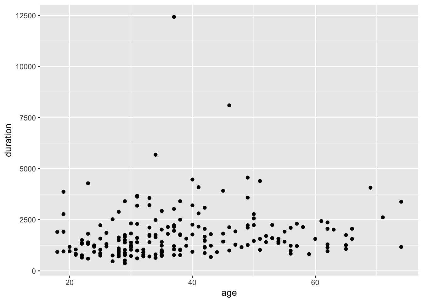
# ggplot() functions takes a tibble (in this case AmE_demo) as its first argument.
# Different plots have their own basic shape, 'geom'. Here it is geom_point which gives us a scatter plot.
Aesthetic mappings
# We can specify aesthetic mappings inside a geom or inside the main ggplot(). In the above cell we did it inside the geom. Now let's try the other way:
ggplot(AmE_demo, aes(x = age, y = duration)) +
    geom_point()
# And it gives us the same thing. But specifying aesthetic mappings inside the main ggplot() allows multiple geoms to draw from the same mappings, which will be handy when we add more stuff to our plot later.Now let’s try making the points into the participants’s gender and see what happends when we replace geom_point with geom_text.
#ggplot(AmE_demo, aes(x = age, y = duration)) +
    #geom_text()

# It gives us an error! This is because geom_text requires additional aesthetic mapping. We need to know which column is the label.

# Error in geom_text() :
#ℹ Error occurred in the 1st layer.
#Caused by error in `compute_geom_1()`:
#! `geom_text()` requires the following missing aesthetics: label.
# We need to specify what the label is:
ggplot(AmE_demo, aes(x = age, y = duration, label = gender)) +
geom_text()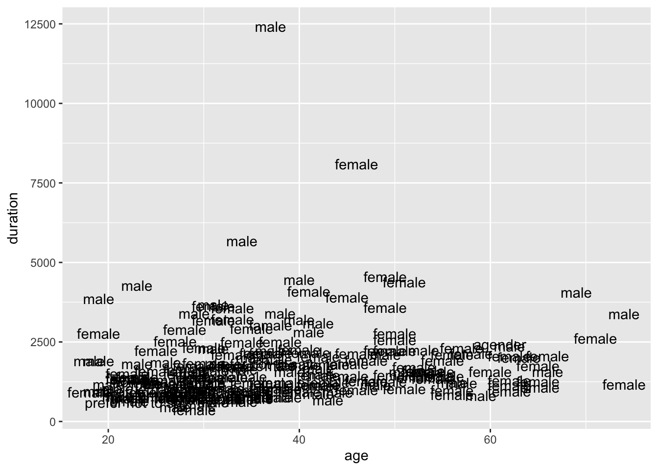
# Not sure if this type of graph will be useful but I guess the point is, we need to specify 'label' in when we use geom_text :)To save a plot:
ggsave("geom_text.png", width = 8, height = 6)If we want to make a two-plot arrangement, we can use gridExtra package:
plot1 <- ggplot(AmE_demo, aes(x = age, y = duration)) +
    geom_point()

plot2 <- ggplot(AmE_demo, aes(x = age, y = duration, label = gender)) +
    geom_text()

# Plot doublt plot:

library(gridExtra)
Attaching package: 'gridExtra'The following object is masked from 'package:dplyr':
combinegrid.arrange(plot1, plot2, ncol = 2)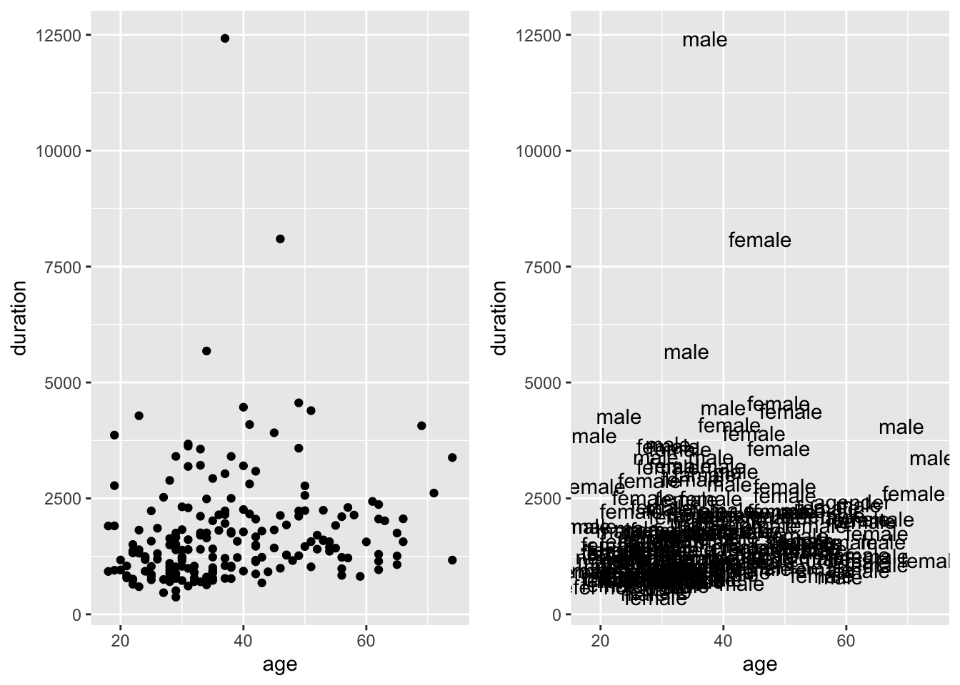
# ncol specifies a plot arrangement with how many columns

# Yes the graph is very ugly but just for demonstration :)
===============================================================================================================
2.5 Piping with magrittr
“Imagine a conveyor belt where the output of one function serves as the input to another
function.” (Winter, 2020, p. 37)
Let’s say we want to plot a graph for those who were over 40 years of age:
AmE_demo %>%
  filter(age > 40) %>%
  ggplot(aes(x = age, y = duration)) +
    geom_point()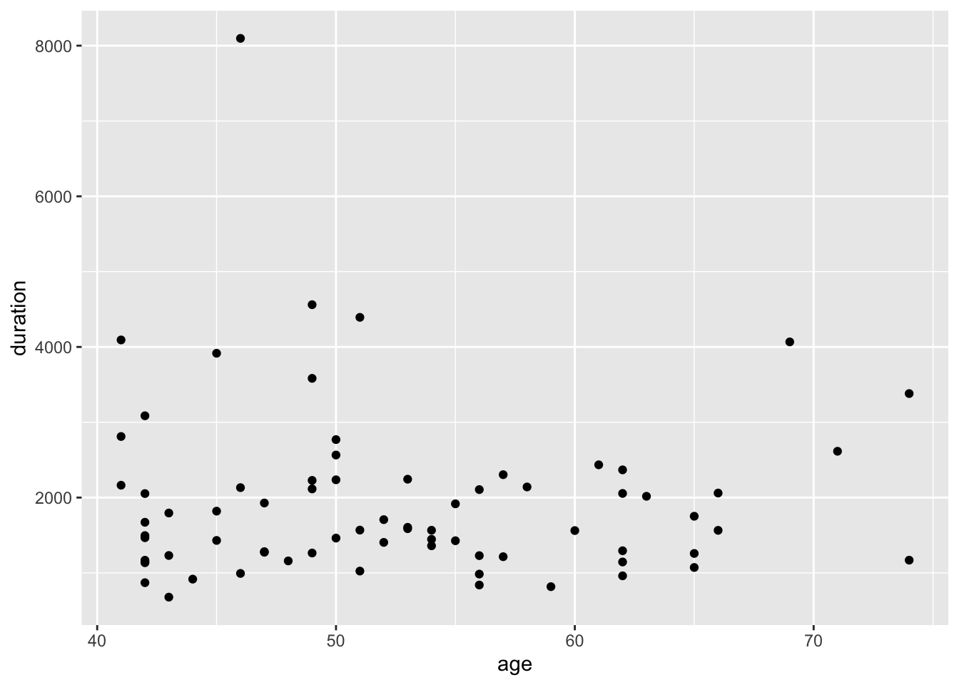
# Here, we first pipe the filter() to the AmE_demo tibble. Then we pipe the ggplot() function to the filtered tibble.

# Winter used geom_text() but it just doesn't look pleasing to my eyes :)
===============================================================================================================
2.6 A more extensive example
In this section, Winter talks about a study on iconicity (Winter et al. 2017). I will try to apply what he did using my own example. In Winter’s example, there were more numerical variables but in mine, most of the variables were categorical.
Let’s load some more data.
AmE_data <- read_csv("AmE_data.csv") %>%
  rename(id = ResponseID)
Rows: 648 Columns: 3
── Column specification ────────────────────────────────────────────────────────
Delimiter: ","
chr (3): ResponseID, context, irony_type
ℹ Use `spec()` to retrieve the full column specification for this data.
ℹ Specify the column types or set `show_col_types = FALSE` to quiet this message.AmE_data# A tibble: 648 × 3
id context irony_type
<chr> <chr> <chr>
1 R_1QK2lCsuAWneFft NEWS_NEG Not ironic
2 R_3ke8DpF2H8JT9Dw DATE_NEG Not ironic
3 R_1nwx6Wmj5DPm5Ao STUDS_NEG Understatement
4 R_1nwx6Wmj5DPm5Ao STUDS_NEG Sarcasm
5 R_3ke8DpF2H8JT9Dw EXP_NEG Not ironic
6 R_63gbAlSDNNkcTsn STUDS_NEG Hyperbole
7 R_37xLIj9QOwOaVnP NEWS_NEG Not ironic
8 R_5mPppAWzoa9LPxO STUDS_NEG Not ironic
9 R_5NLaD0kaEUTbBAt OLDMAN_NEG Not ironic
10 R_7RsbYRr3XGqN8qa OLDMAN_NEG Rhetorical question
# ℹ 638 more rows# What does this tibble tell us?
# This is data from a survey where people were given different scenarios and they produced irony/sarcasm accordingly.We are going to use AmE_demo as well.
AmE_demo# A tibble: 202 × 10
duration id age gender ed L1 birthplace residence abroad where
<dbl> <chr> <dbl> <chr> <chr> <chr> <chr> <chr> <chr> <chr>
1 704 R_1aDoqa… 28 female Unde… Engl… USA Philadel… Yes Japa…
2 751 R_8BbNFu… 27 female unde… engl… united st… helena No <NA>
3 958 R_5YmJvQ… 20 male Some… Engl… United St… San Diego No <NA>
4 1562 R_4jGPhl… 60 female unde… Engl… United St… New Orle… No <NA>
5 1011 R_1CJjsz… 38 female Post… Engl… New Jersey Howell No <NA>
6 1072 R_2j1YU3… 65 female Mast… Engl… Hershey, … Newville… Yes N. I…
7 1159 R_46gLJt… 30 female Asso… Engl… America Grand Ra… No <NA>
8 509 R_7CTqax… 29 female unde… engl… new york Brooklyn No <NA>
9 1757 R_1egBkg… 33 female bach… Engl… Alabama, … Ellenwoo… Yes Kore…
10 1229 R_1qwaXr… 56 male Mast… Engl… Vietnam Champaig… Yes Saud…
# ℹ 192 more rowsLet’s join the two tibbles together and then plot sth.
AmE <- left_join(AmE_data, AmE_demo)Joining with `by = join_by(id)`AmE# A tibble: 648 × 12
id context irony_type duration age gender ed L1 birthplace
<chr> <chr> <chr> <dbl> <dbl> <chr> <chr> <chr> <chr>
1 R_1QK2lCsuAW… NEWS_N… Not ironic 1672 42 male high… Engl… United St…
2 R_3ke8DpF2H8… DATE_N… Not ironic 1659 29 male unde… engl… Ghana
3 R_1nwx6Wmj5D… STUDS_… Understat… 1574 39 male unde… Engl… New York …
4 R_1nwx6Wmj5D… STUDS_… Sarcasm 1574 39 male unde… Engl… New York …
5 R_3ke8DpF2H8… EXP_NEG Not ironic 1659 29 male unde… engl… Ghana
6 R_63gbAlSDNN… STUDS_… Hyperbole 1495 42 male Some… Engl… Louisiana
7 R_37xLIj9QOw… NEWS_N… Not ironic 466 27 male unde… Engl… United St…
8 R_5mPppAWzoa… STUDS_… Not ironic 2811 41 male Unde… Engl… United St…
9 R_5NLaD0kaEU… OLDMAN… Not ironic 4467 40 male Post… Engl… United St…
10 R_7RsbYRr3XG… OLDMAN… Rhetorica… 1826 30 female trad… engl… united st…
# ℹ 638 more rows
# ℹ 3 more variables: residence <chr>, abroad <chr>, where <chr>Now let’s try just looking at the data where participants gave a valid ironic response:
AmE_irony <- AmE %>%
  filter(!irony_type %in% c("Not ironic", "DNFI")) %>%
  arrange(context)

AmE_irony
# A tibble: 594 × 12
id context irony_type duration age gender ed L1 birthplace
<chr> <chr> <chr> <dbl> <dbl> <chr> <chr> <chr> <chr>
1 R_5CqZMzZThy… DATE_N… Rhetorica… 1566 54 female high… Engl… New Jerse…
2 R_2rixwdZktg… DATE_N… Rhetorica… 1294 62 female High… Engl… 1961
3 R_1P7a946agj… DATE_N… Rhetorica… 2106 56 female Unde… Engl… Charlesto…
4 R_5t001Gnwb8… DATE_N… Sarcasm 5680 34 male bach… Engl… United St…
5 R_3jCYDGIJOW… DATE_N… Sarcasm 1159 48 male Post… Engl… United St…
6 R_37xLIj9QOw… DATE_N… Sarcasm 466 27 male unde… Engl… United St…
7 R_7JlBZHXmHF… DATE_N… Sarcasm 760 22 female unde… engl… united st…
8 R_7JlBZHXmHF… DATE_N… Understat… 760 22 female unde… engl… united st…
9 R_5MYVwpwAlH… DATE_N… Sarcasm 2231 25 female Post… Engl… Tallahass…
10 R_5MYVwpwAlH… DATE_N… Understat… 2231 25 female Post… Engl… Tallahass…
# ℹ 584 more rows
# ℹ 3 more variables: residence <chr>, abroad <chr>, where <chr>Let’s plot sth :) Maybe a historgram on age?
AmE_age <- AmE_irony %>%
  ggplot(aes(x = age)) +
  geom_histogram(binwidth = 5, fill = "limegreen", color = "white") +
  theme_minimal()

AmE_age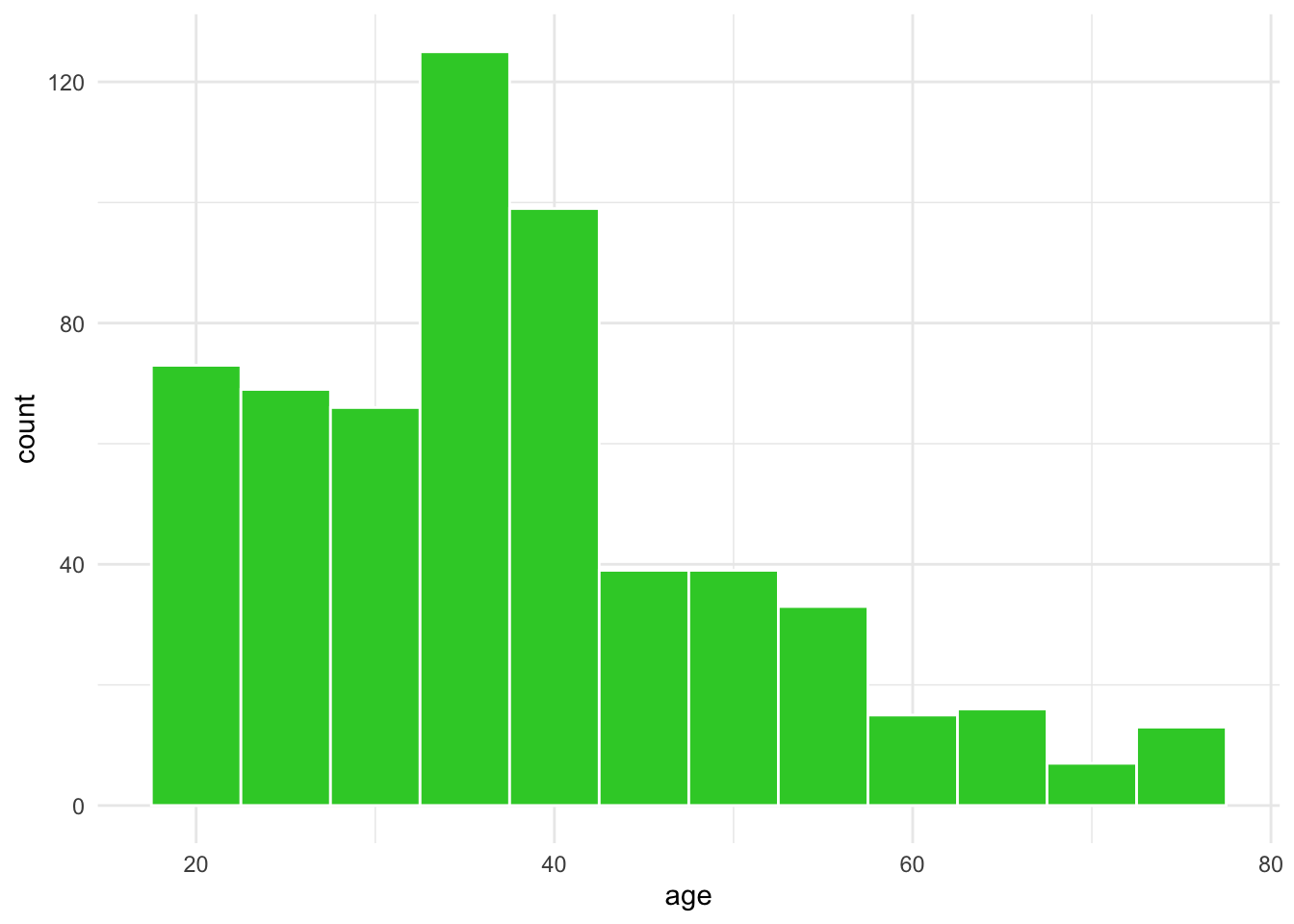
What if we want to see which type of irony was produced the most?
AmE_irony_count <- AmE_irony %>%
  count(irony_type) %>%
  ggplot(aes(x = irony_type, y = n)) +
  geom_bar(stat = 'identity', fill = "hotpink") +
    theme_minimal()

AmE_irony_count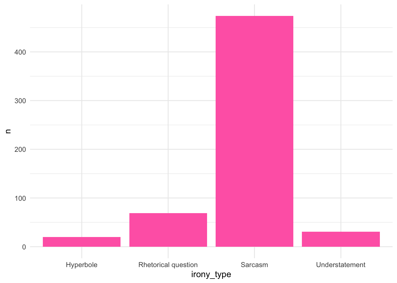
# "You need to specify the additional argument stat = 'identity'. This is because the geom_bar() function likes to perform its own statistical computations by default (such as counting). With the argument stat = 'identity', you instruct the function to treat the data as is." (Winter, 2020, p. 44)

# If we don't specify stat = 'identity' but instead with 'count':
df <- AmE_irony %>%
  count(irony_type) %>%
  ggplot(aes(irony_type)) +
  geom_bar(stat = 'count', fill = "limegreen") +
  theme_minimal()

df
What if we want to plot the number of sarcasm produced in each context?
AmE_sarcasm_count <- AmE_irony %>%
  filter(irony_type == "Sarcasm") %>%
  count(context) %>%
  ggplot(aes(x = context, y = n, fill = context)) +
  geom_col() +
  theme_minimal()

AmE_sarcasm_count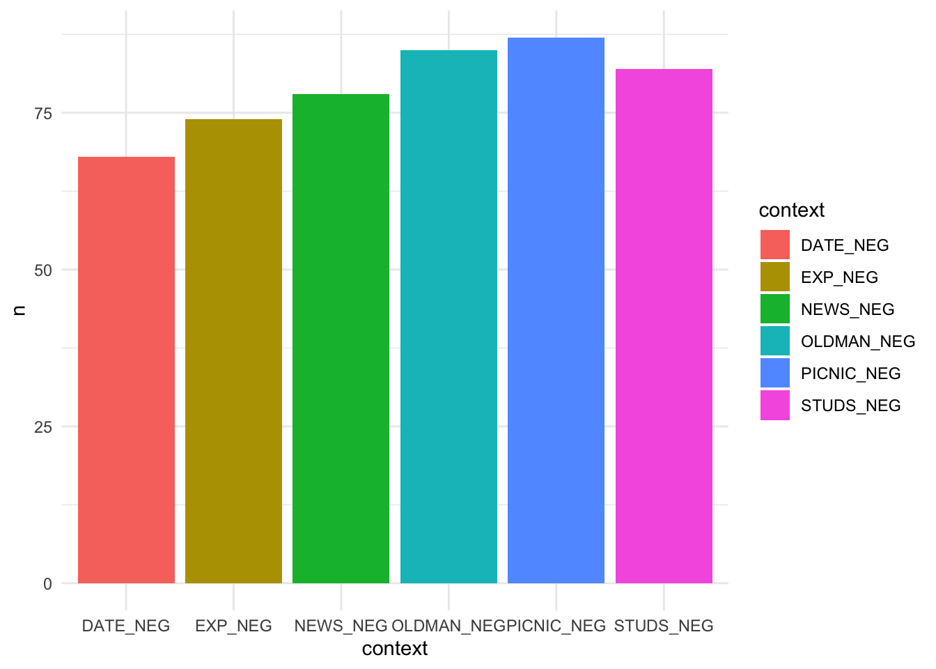
# geom_col() uses stat = "identity" Now let’s try to plot a boxplot with age and irony type to see whether certain irony types are produced more by younger/older participants:
AmE_age <- AmE_irony %>%
  ggplot(aes(x = irony_type, y = age, fill = irony_type)) +
  geom_boxplot() +
  theme_minimal()

AmE_age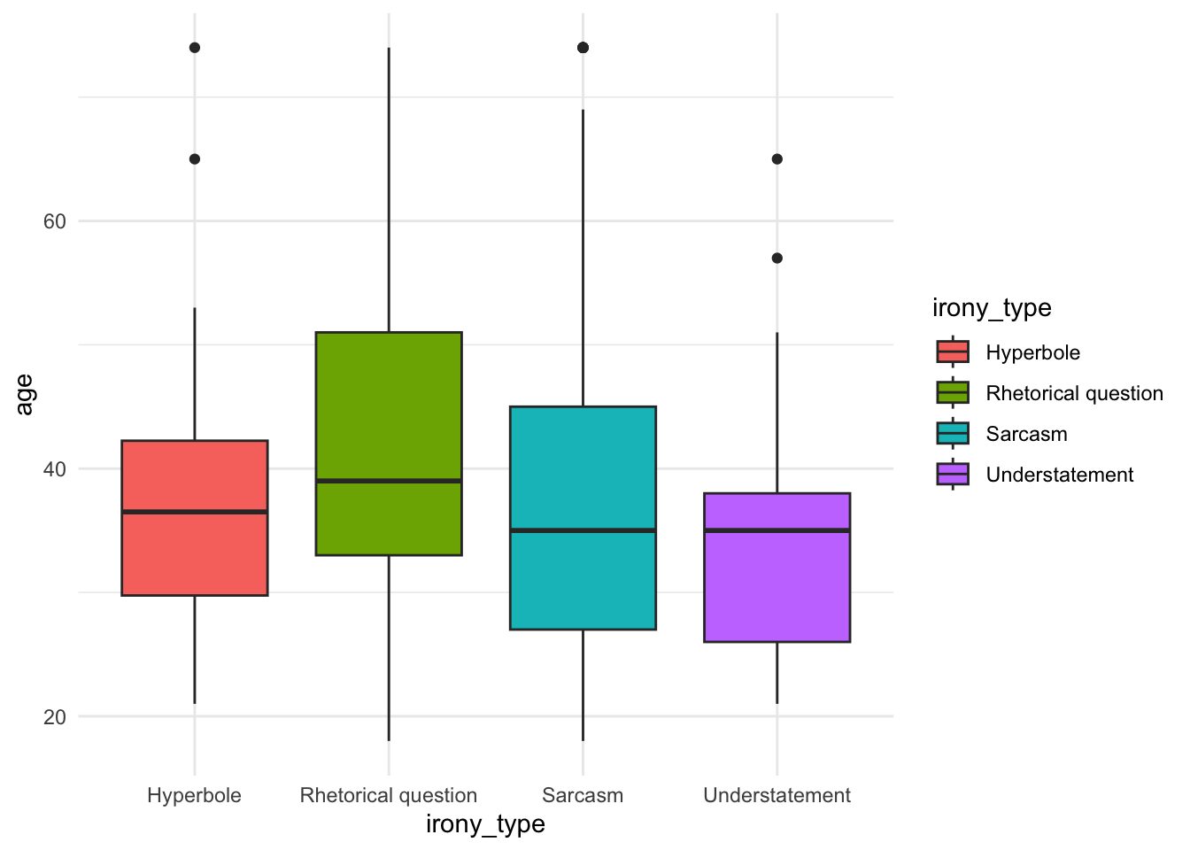
Download
Use this link to download this .qmd file and associated data.