Ch4.6-4.9 Setting up a Simple Linear Model

Author

Qi Yi

Published

October 8, 2025

In today’s session, we will cover

how to use library(tidyverse) library(broom) library(ggplot)
setting up a simple linear model,
creating a scatterplot with a regression line
Intercept placeholder

Definitions

Q1. What is a Linear Regression Model?

To answer this question, we need to understand three terminologies, “linear”, “regression”, and “model”. The non-mathematical human-language answers would be:

A model can be seen as a mathematical representation of the relationship or association between two or more variables. It consists of two components, variables and parameters, or coefficients (they are the estimate of parameters) (Heumann et al., p.269). A model can also be considered as a mathematical construct that we use to interpret the mechanism of generating the observed data (Rencher et al., 2008, p.2).
Whether the model is linear or non-linear is indeed a broad and difficult question. Simply saying, it is determined by the parameters (or the coefficients), for example, if the parameter is \(β_1^{2}\) , the model is non-linear (Heumann et al., 2022, p.269).
Regression analysis is used to analyze a relationship between two or more variables in which one of the variables can be predicted or explained by the information given by the other variables (Mohr et al., 2022, p.302).

Q2. What is simple linear regression?

In a simple linear regression, there is only one variable, x, to predict the response of y. The model can be written as

\[y=b_0+b_1x+e\]

\(b_0\) is the intercept, \(b_1\) is the coefficient.

A regression line can be used to describe how the dependent variabley changes as independent variable x changes. The process of modeling is to find out the most “suitable” regression coefficients. In another word, to find the best fitted line among the data points, and draw a regression line that leads to the least squares of errors.

Part 2: Model Setup

Based on the given equation, let’s start to set up a simply linear regression

library(tidyverse)

── Attaching core tidyverse packages ──────────────────────── tidyverse 2.0.0 ──
✔ dplyr     1.1.4     ✔ readr     2.1.5
✔ forcats   1.0.0     ✔ stringr   1.5.1
✔ ggplot2   3.5.1     ✔ tibble    3.2.1
✔ lubridate 1.9.3     ✔ tidyr     1.3.1
✔ purrr     1.0.2     
── Conflicts ────────────────────────────────────────── tidyverse_conflicts() ──
✖ dplyr::filter() masks stats::filter()
✖ dplyr::lag()    masks stats::lag()
ℹ Use the conflicted package (<http://conflicted.r-lib.org/>) to force all conflicts to become errors

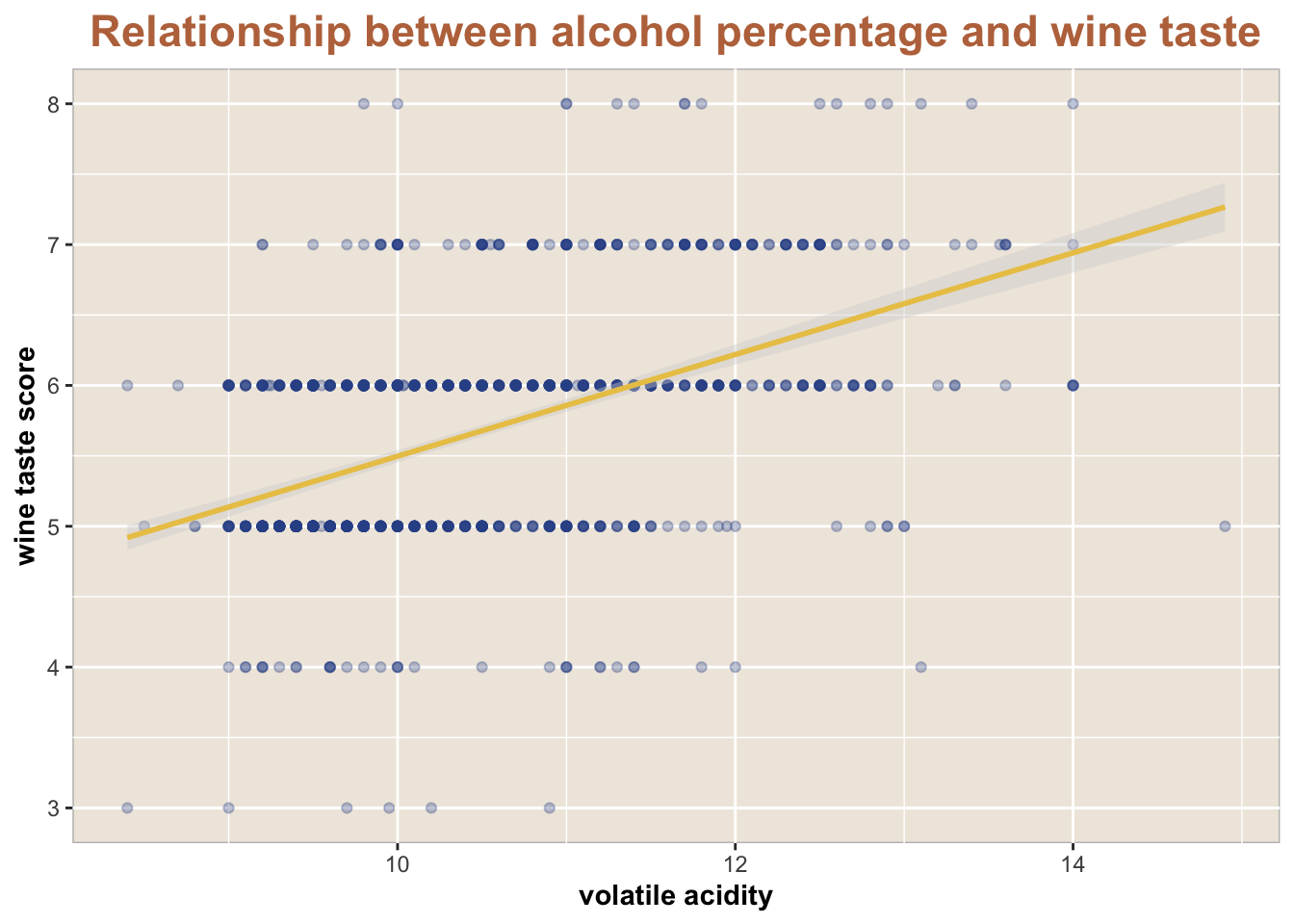
The First Model: The relationship between alcohol percentage in wine and wine taste

Background: The WineQuality.csv dataset was created to investigate the relationship between wine preference and wine physicochemical properties. The data was collected between 2004 and 2007. Samples all came from a unique type of Portugese wine vinho verde from the northwest region of Portugal. Each sample was tasted by three tasters, and the final sensory score was determined by the median of score of these tasters.

The document WineQuality.csv has 13 columns, in which, column 11 shows the percentage of alcohol in each sample (column name= ‘alcohol’, % VOL), column 12 shows the sensory score (column name=‘quality’ ) of the sample. When evaluating, score ranged from 0-10, 0 meant very bad 👎 , 10 meant excellent 🤤.

🐾 Step 1- load the csv file

# Load data
wine_quality <- read_csv('WineQuality.csv')

Rows: 1143 Columns: 13
── Column specification ────────────────────────────────────────────────────────
Delimiter: ","
dbl (13): fixed acidity, volatile acidity, citric acid, residual sugar, chlo...

ℹ Use `spec()` to retrieve the full column specification for this data.
ℹ Specify the column types or set `show_col_types = FALSE` to quiet this message.

colnames(wine_quality)

 [1] "fixed acidity"        "volatile acidity"     "citric acid"         
 [4] "residual sugar"       "chlorides"            "free sulfur dioxide" 
 [7] "total sulfur dioxide" "density"              "pH"                  
[10] "sulphates"            "alcohol"              "quality"             
[13] "Id"

wine_quality

# A tibble: 1,143 × 13
   `fixed acidity` `volatile acidity` `citric acid` `residual sugar` chlorides
             <dbl>              <dbl>         <dbl>            <dbl>     <dbl>
 1             7.4               0.7           0                 1.9     0.076
 2             7.8               0.88          0                 2.6     0.098
 3             7.8               0.76          0.04              2.3     0.092
 4            11.2               0.28          0.56              1.9     0.075
 5             7.4               0.7           0                 1.9     0.076
 6             7.4               0.66          0                 1.8     0.075
 7             7.9               0.6           0.06              1.6     0.069
 8             7.3               0.65          0                 1.2     0.065
 9             7.8               0.58          0.02              2       0.073
10             6.7               0.58          0.08              1.8     0.097
# ℹ 1,133 more rows
# ℹ 8 more variables: `free sulfur dioxide` <dbl>,
#   `total sulfur dioxide` <dbl>, density <dbl>, pH <dbl>, sulphates <dbl>,
#   alcohol <dbl>, quality <dbl>, Id <dbl>

range(wine_quality$quality)

[1] 3 8

🐾 Step 2 - Create a simple linear regression model

Before creating a simple linear regression model, let’s set up a null model.

What does the intercept mean in the null model? – It means the average score (mean of the dependent variable).

model_null <- lm(quality~1, data =wine_quality)
model_null


Call:
lm(formula = quality ~ 1, data = wine_quality)

Coefficients:
(Intercept)  
      5.657

Why is there “1” in the null model?

1 represents the intercept place holder. In R, the shorthand notation ‘y ~ x’ fits the model corresponding to the formula y ~ 1+x. The intercept is by default. Therefore, when building a null model, we use y ~ 1.

model1 <- lm(quality~alcohol,data=wine_quality)
model1


Call:
lm(formula = quality ~ alcohol, data = wine_quality)

Coefficients:
(Intercept)      alcohol  
      1.887        0.361

\[ Wine\ taste\ score = 1.887 + 0.361 * alcohol\ percentage \]

res<- residuals(model1)
hist(res,xlab="residuals")

🐾 Step 3 - Produce a scatterplot of years of experience versus salary

By using geom_smooth(), we can plot a linear model by specifying the argument method='lm'.

The gray ribbon around the regression line is the ‘95% confidence interval’ (see Chapter 9)

ggplot(wine_quality,aes(x=alcohol,y=quality))+
  geom_point(alpha=0.3,color="#314F94")+
  geom_smooth(method='lm',formula = y ~ x,color='#EAC655',fill = "lightgrey")+
  labs(x="volatile acidity", y="wine taste score",title="Relationship between alcohol percentage and wine taste")+
  theme(plot.title = element_text(size = 17, face = "bold",hjust = 0.5, color ='#BC734A'),
        axis.title = element_text(size = 11, face = "bold"),
        panel.background = element_rect(fill = "#EFE8DF", color = 'grey'))

🐾 Step 4 - Retrieve information from the model

We can use fitted() to retrieve the model’s fitted values.

5.280798 is the prediction for the first data point.

head(fitted(model1))

       1        2        3        4        5        6 
5.280798 5.425214 5.425214 5.425214 5.280798 5.280798

#wine_quality$quality[1]
#wine_quality$quality[1]-head(fitted(model1))[1]

We can use residuals() to retrieve the model’s fitted residuals

head(residuals(model1))

         1          2          3          4          5          6 
-0.2807980 -0.4252143 -0.4252143  0.5747857 -0.2807980 -0.2807980

Use summary() to get a coefficient table which includes useful summary statistics for the overall model fit.

summary(model1)


Call:
lm(formula = quality ~ alcohol, data = wine_quality)

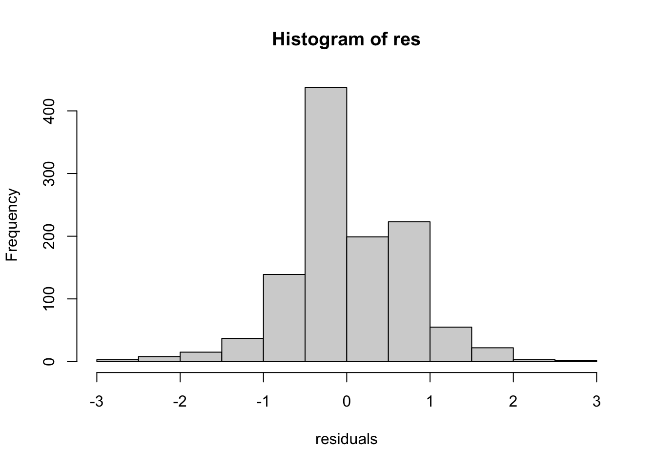
Residuals:
    Min      1Q  Median      3Q     Max 
-2.8224 -0.4000 -0.1725  0.5152  2.5748 

Coefficients:
            Estimate Std. Error t value Pr(>|t|)    
(Intercept)  1.88701    0.20240   9.323   <2e-16 ***
alcohol      0.36104    0.01928  18.727   <2e-16 ***
---
Signif. codes:  0 '***' 0.001 '**' 0.01 '*' 0.05 '.' 0.1 ' ' 1

Residual standard error: 0.7051 on 1141 degrees of freedom
Multiple R-squared:  0.2351,    Adjusted R-squared:  0.2344 
F-statistic: 350.7 on 1 and 1141 DF,  p-value: < 2.2e-16

#summary(model1)$r.squared

Use coef() to retrieve the coefficients of a linear model. The output is a vector.

coef(model1)

(Intercept)     alcohol 
   1.887013    0.361041

coef(model1)[1]

(Intercept) 
   1.887013

# alternative way of indexing by name
coef(model1)['alcohol']

 alcohol 
0.361041

# Calculate the fitted value for an x-value of 11
coef(model1)['(Intercept)'] + coef(model1)['alcohol']*11

(Intercept) 
   5.858464

🐾 Step 5 - Using the setup model to predict values

Alternatively, we can also generate predictions for a given sequence of numbers by using predict() .

Note

predict(object, newdata)

seq(from= , to= , by= )

# Generate prediction for a sequence of numbers by using the model
alcohol_values<-seq(from=11, to=13, by= 0.2)
mypreds<-tibble(alcohol=alcohol_values)
mypreds$score<- predict(model1,newdata=mypreds)
mypreds

# A tibble: 11 × 2
   alcohol score
     <dbl> <dbl>
 1    11    5.86
 2    11.2  5.93
 3    11.4  6.00
 4    11.6  6.08
 5    11.8  6.15
 6    12    6.22
 7    12.2  6.29
 8    12.4  6.36
 9    12.6  6.44
10    12.8  6.51
11    13    6.58

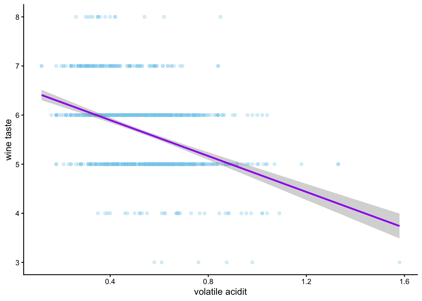
The Second Model: The relationship between volatile acidity in wine and wine taste

Now let’s use set up another simple linear model by using library(broom).

This time we want to look into the relationship between volatile acidity and wine taste.

Fun fact: What is Volatile Acidity (VA)? 🍷

VA measures the of amount of acids in wine that evaporate easily (mainly acetic acid). Excessive levels of VA will effect the taste of the wine and are considered as a wine fault. A small amount can add complexity. It is a key quality control measure in winemaking.

VA Unit: g(acetic acid)/dm3, means grams of acetic acid per cubic decimeter

🐾 Step 1 - Load data, set up a null model

newdf<- tibble(wine_quality$`volatile acidity`, wine_quality$quality)
null_model2 <- lm(wine_quality$quality~1, data=newdf)
null_model2 # Null model gives us the mean of y


Call:
lm(formula = wine_quality$quality ~ 1, data = newdf)

Coefficients:
(Intercept)  
      5.657

🐾 Step 2 - Set up a simple linear model

# Load raw data
library(broom)


new_model<- lm(wine_quality$quality~wine_quality$`volatile acidity`, data=newdf)

ggplot(wine_quality,aes(x=wine_quality$`volatile acidity`,y=wine_quality$quality))+
  geom_point(alpha=0.3,color="skyblue")+
  geom_smooth(method='lm',formula = y ~ x,color='purple')+
  theme_classic()+
  labs(x="volatile acidit", y="wine taste")

res2<- residuals(new_model)
hist(res2, xlab ="residuals")

Instead of using summary(), we can use tidy() to provide a model output. The advantage of using tidy()is that its output is a data frame, which allows you to easily index the relevant columns.

tidy(new_model)

# A tibble: 2 × 5
  term                            estimate std.error statistic  p.value
  <chr>                              <dbl>     <dbl>     <dbl>    <dbl>
1 (Intercept)                         6.63    0.0680      97.4 0       
2 wine_quality$`volatile acidity`    -1.83    0.121      -15.1 6.25e-47

# compare with summary(), the latter gives more information
#summary(new_model)

🐾 Step 3 - Extract information from the model output

Though tidy() gives less information about the model compared to summary(), glance() gives detailed model performance.

tidy(new_model)$estimate # this only displays the coefficents of the model

[1]  6.628088 -1.827544

# View model performance
glance(new_model)

# A tibble: 1 × 12
  r.squared adj.r.squared sigma statistic  p.value    df logLik   AIC   BIC
      <dbl>         <dbl> <dbl>     <dbl>    <dbl> <dbl>  <dbl> <dbl> <dbl>
1     0.166         0.165 0.736      227. 6.25e-47     1 -1271. 2548. 2563.
# ℹ 3 more variables: deviance <dbl>, df.residual <int>, nobs <int>

Chapter Conclusions (p.84)

A regression line represents a model of conditional mean, specified by slope and intercept.
Coefficients are the principal outcomes of any regression analysis, allowing to make predictions.
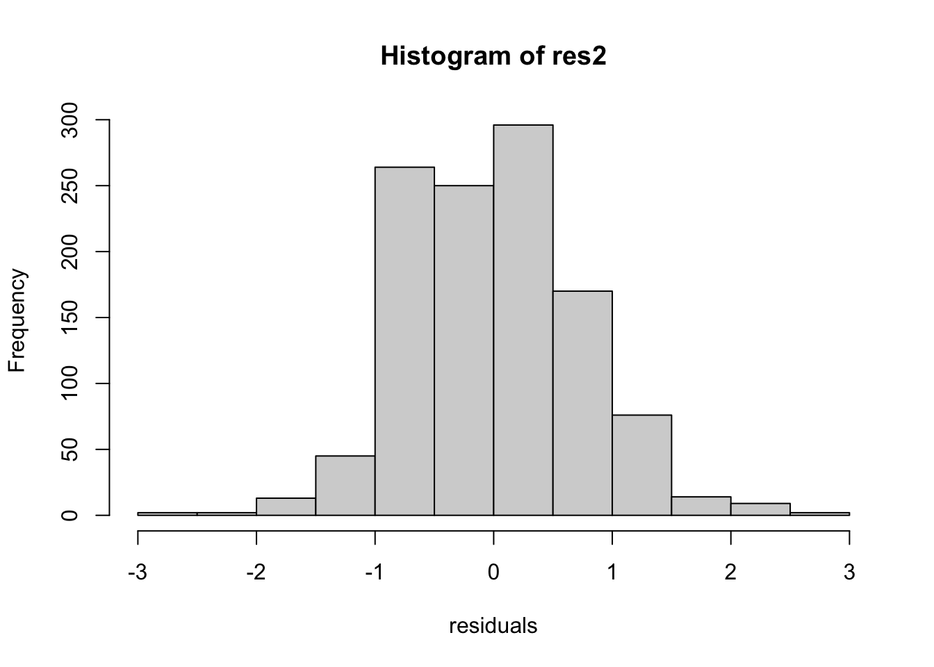
Residuals means the extent by which the observed data points deviate from the fitted values. They are assumed to be normally distributed and homoscedastic (constant variance)
\(R^2\) can be used to evaluate the model performance. It compares the model’s residuals to a null model’s residuals.

References

Heumann, C., Schomaker, M., & Shalabh. (2022). Introduction to statistics and data analysis: with exercises, solutions and applications in R (Second edition.). Springer. https://doi.org/10.1007/978-3-031-11833-3

Mohr, D. L., Wilson, W. J., & Freund, R. J. (2022). Linear regression. In D. L. Mohr, W. J. Wilson, & R. J. Freund (Eds.), Statistical methods (4th ed., pp. 301–349). Academic Press. https://doi.org/10.1016/B978-0-12-823043-5.00007-2

Rencher, A. C., Schaalje, G. B., & Wiley InterScience. (2008). Linear models in statistics (2nd ed.). Wiley-Interscience.r

Downloads

Notebook & Data Download

Download the slide deck version