set.seed(42)
hist(rnorm(500))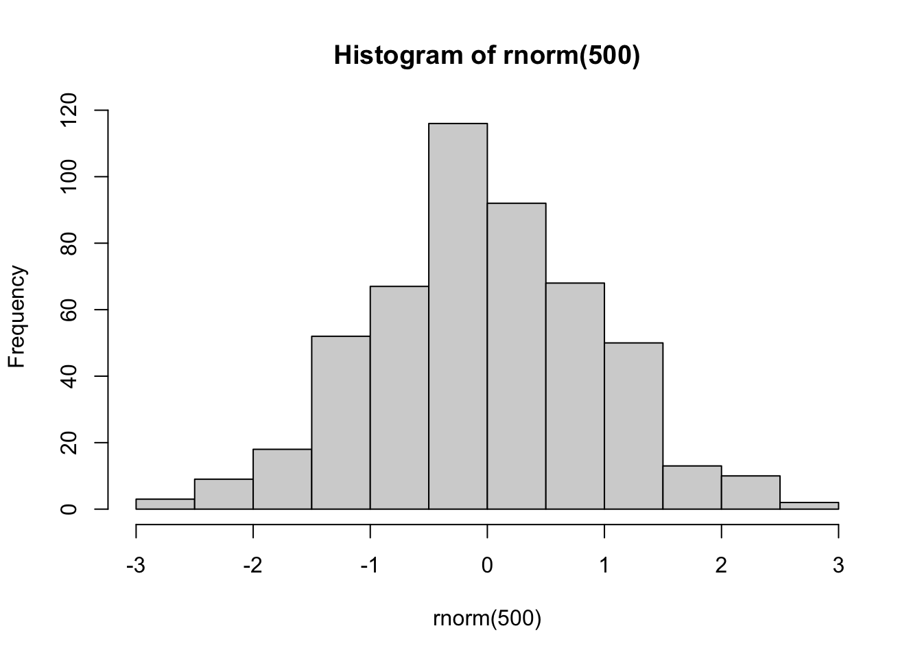
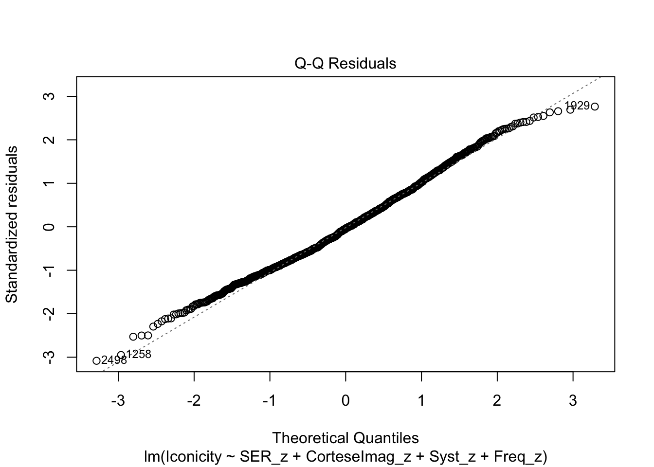
“It’s generally recommended to assess normality and homoscedasticity visually.” p. 109
Two assumptions related to residuals:
We know how to assess normality - we can visualise it with a histogram to look for a relatively even curve on each side of the mean:
set.seed(42)
hist(rnorm(500))
Compare to a random sample of 500 values from 1 to 500 (with replacement)
set.seed(42)
hist(sample(x = 1:500, size = 500, replace = T))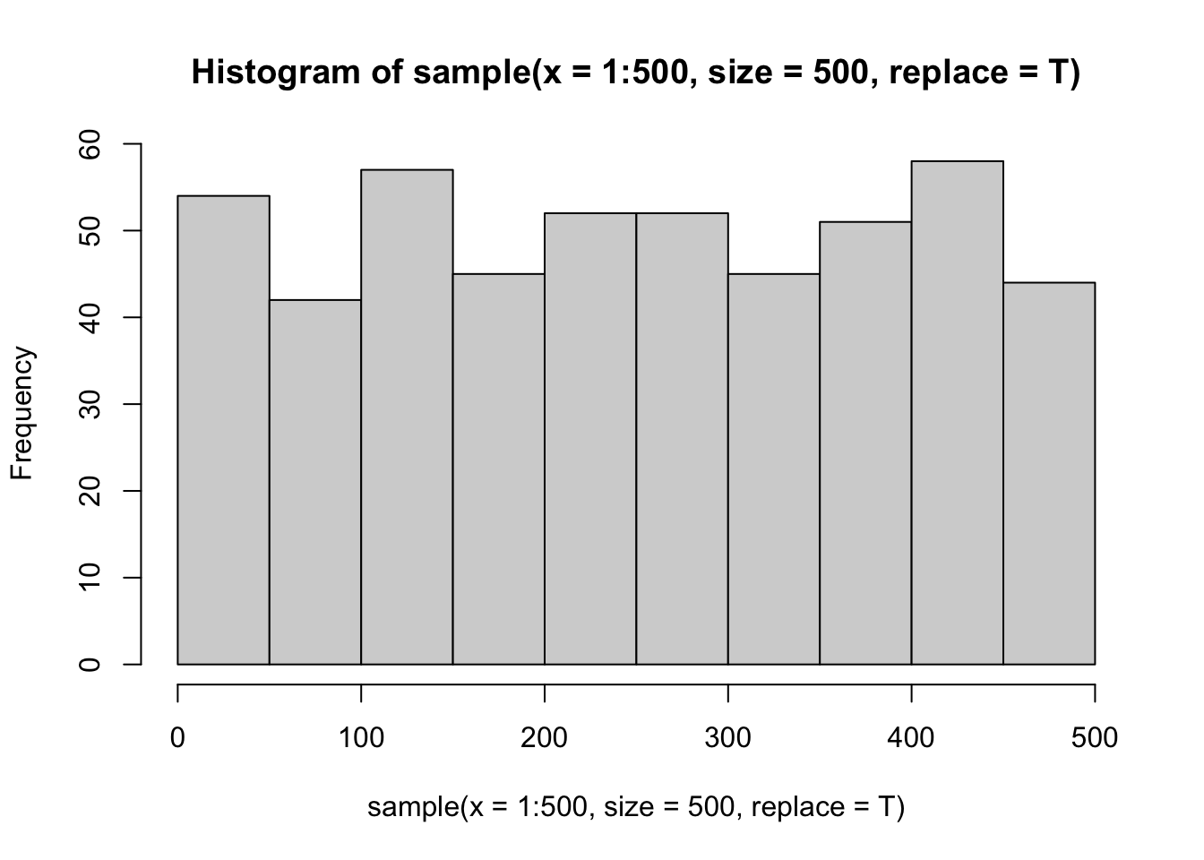
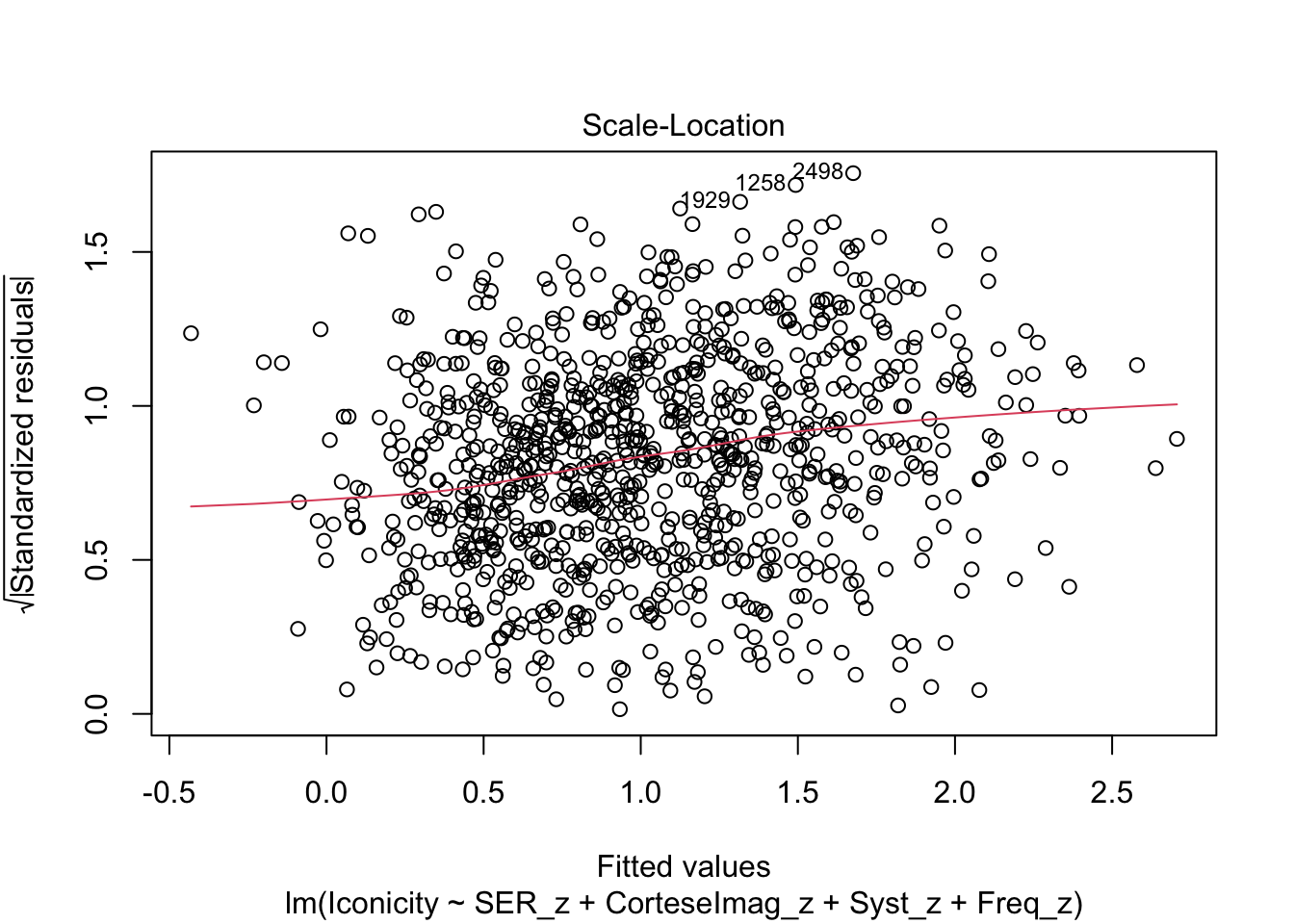
The constant variance assumption relates to visualising the spread of the residuals. The goal is to determine whether the variance in residuals remains constant for different levels of the predictor variables.
The answer from gung here is very helpful
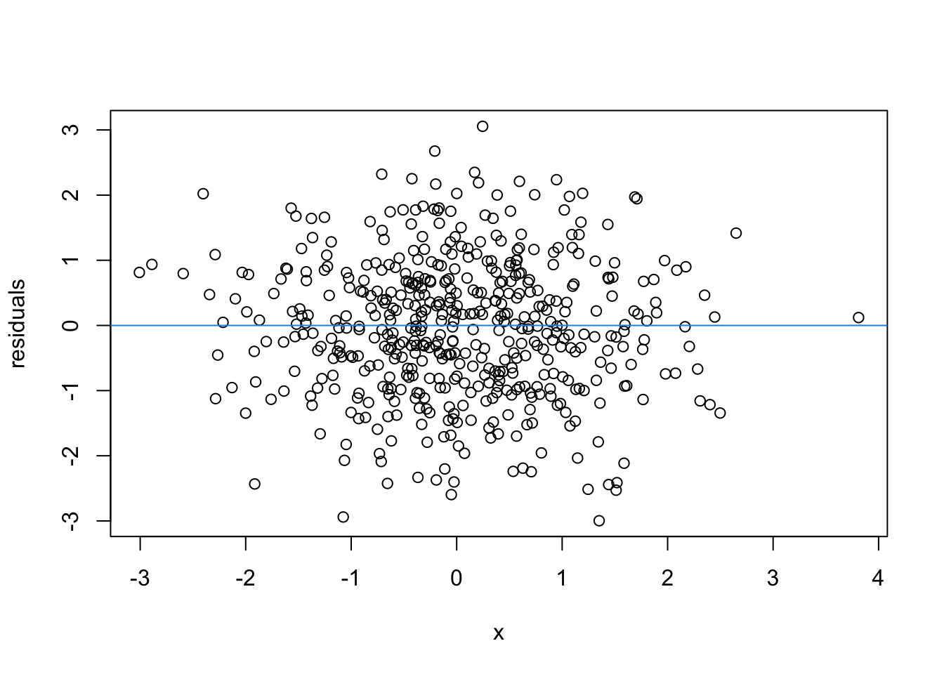
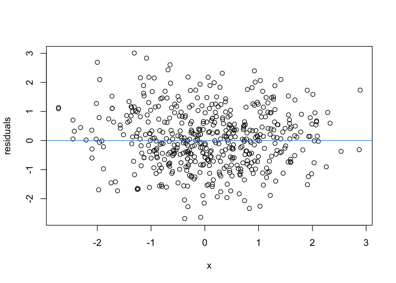
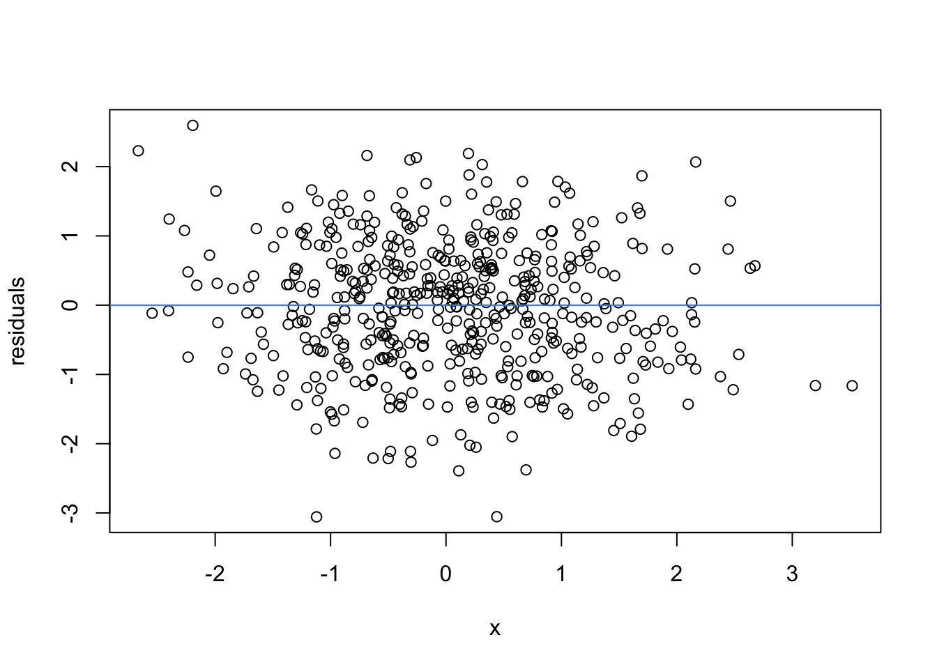
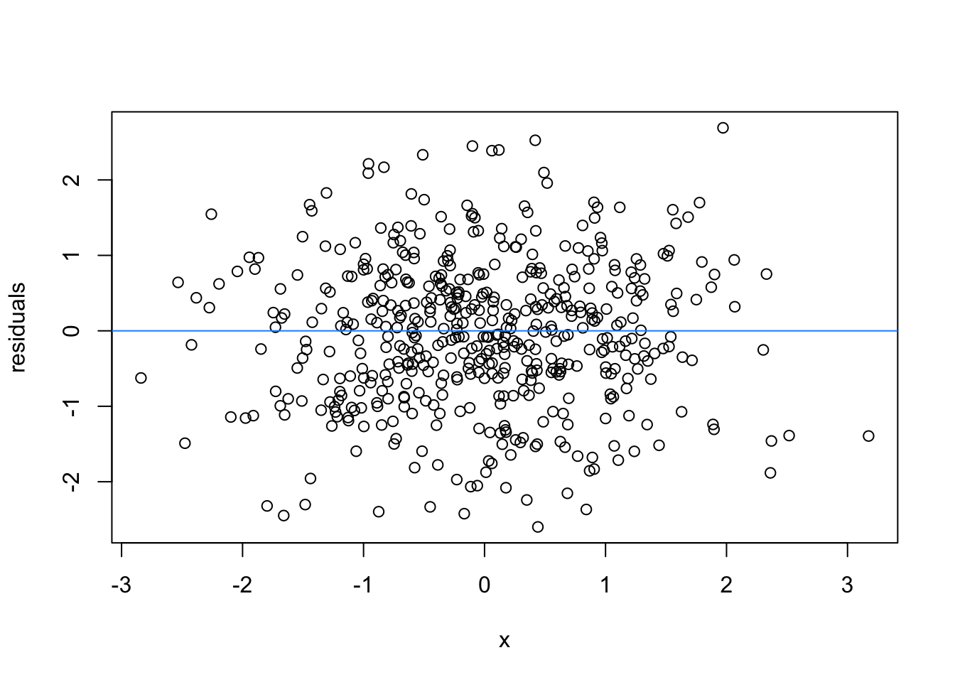
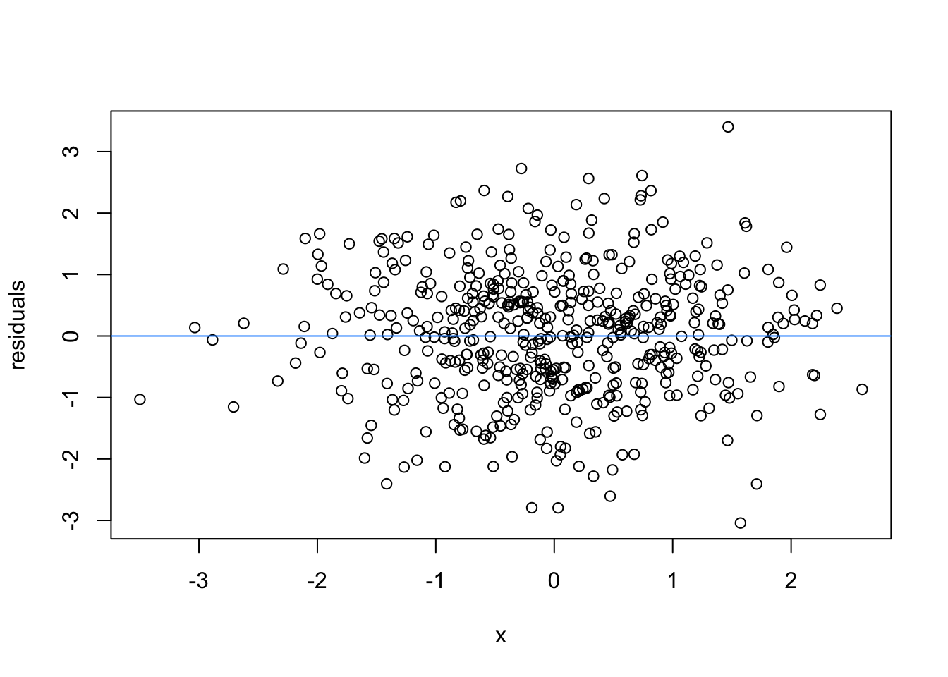
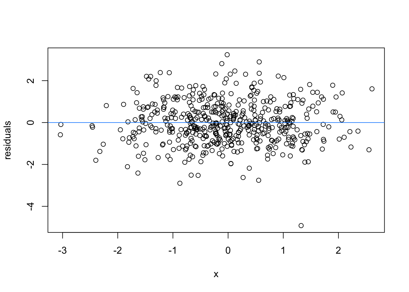
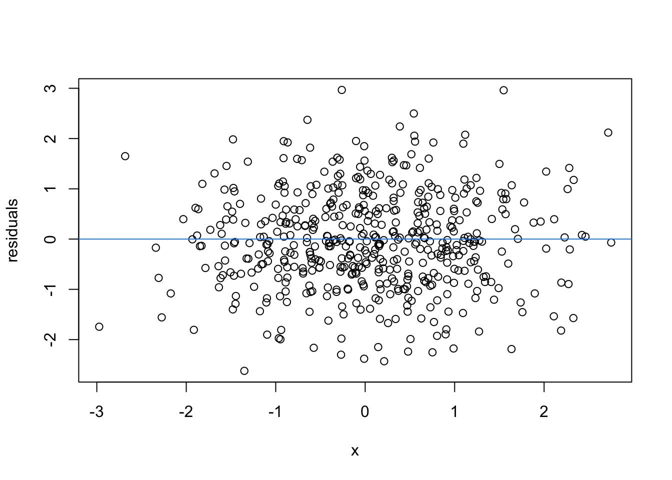
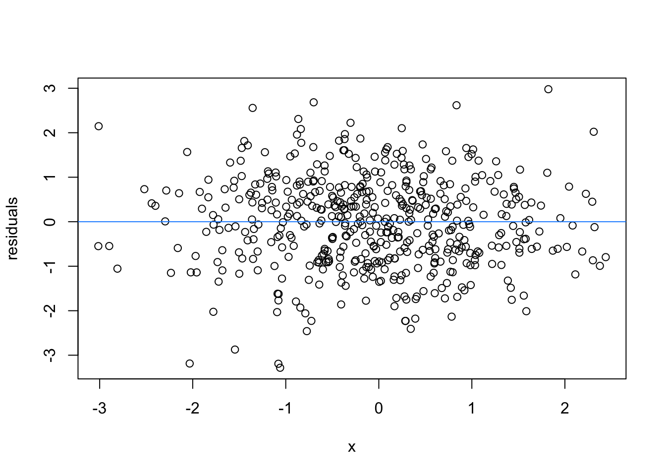
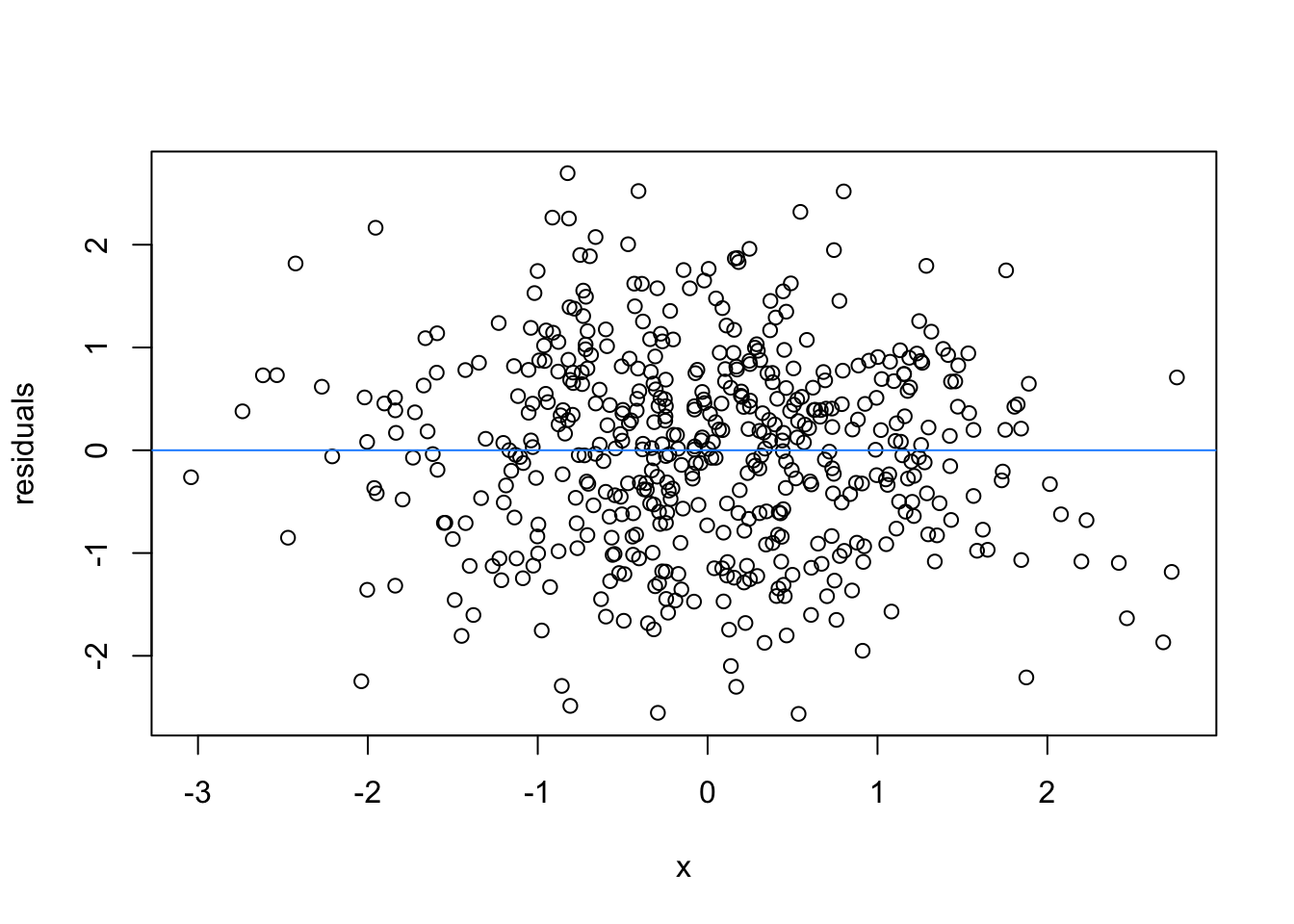
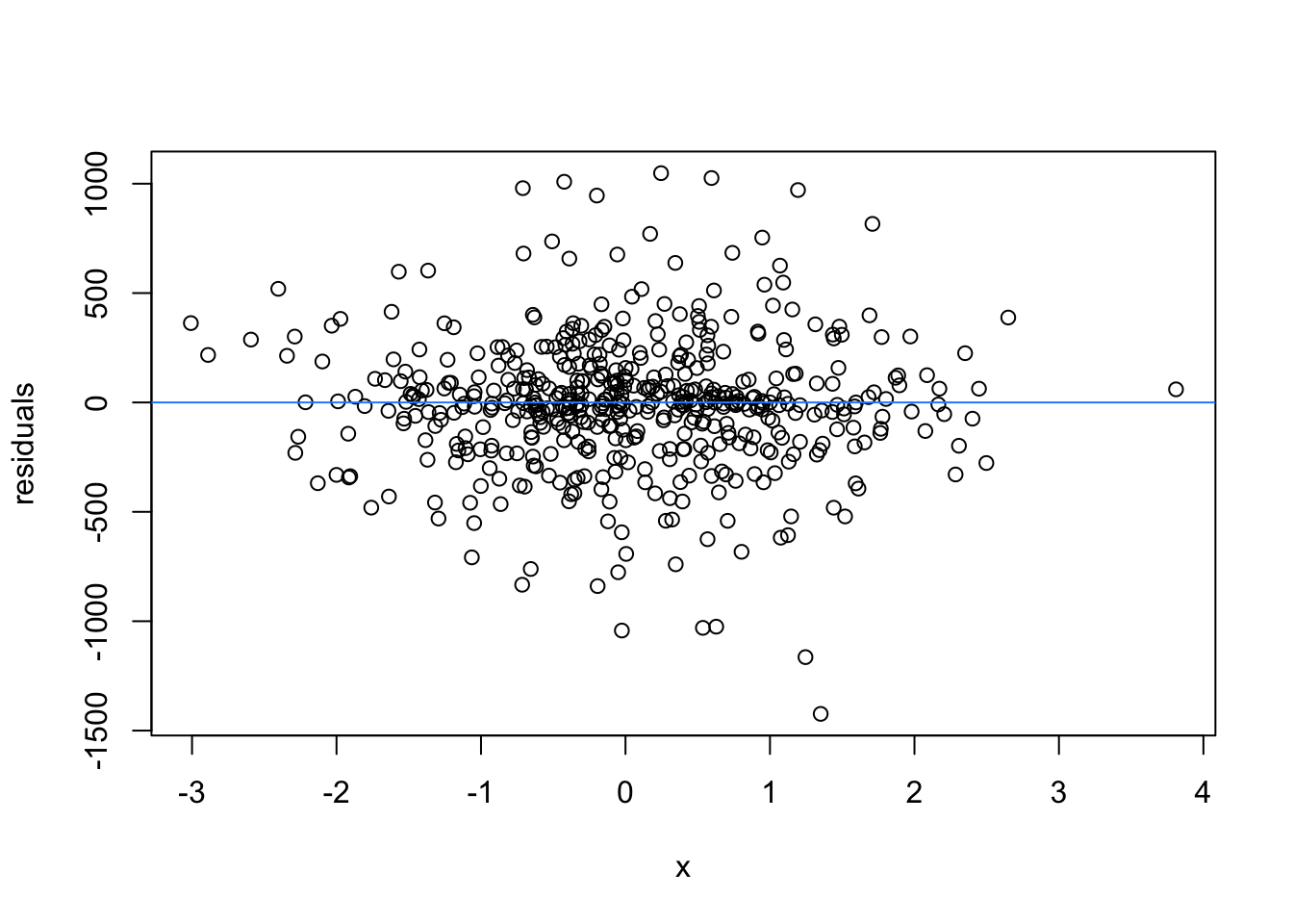
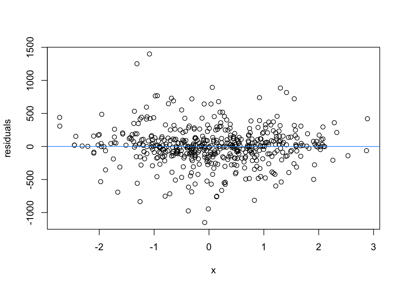
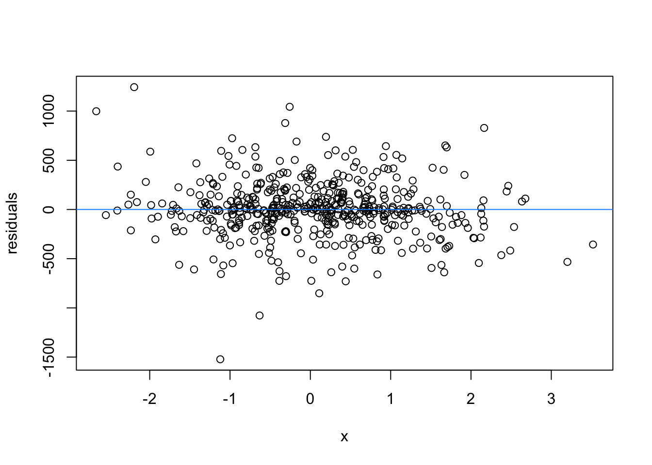
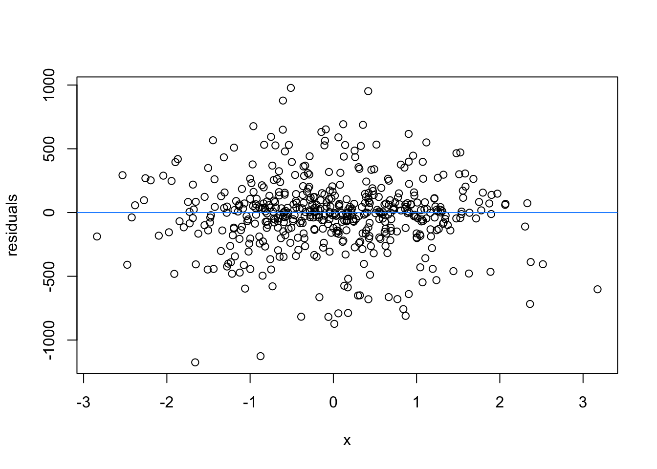
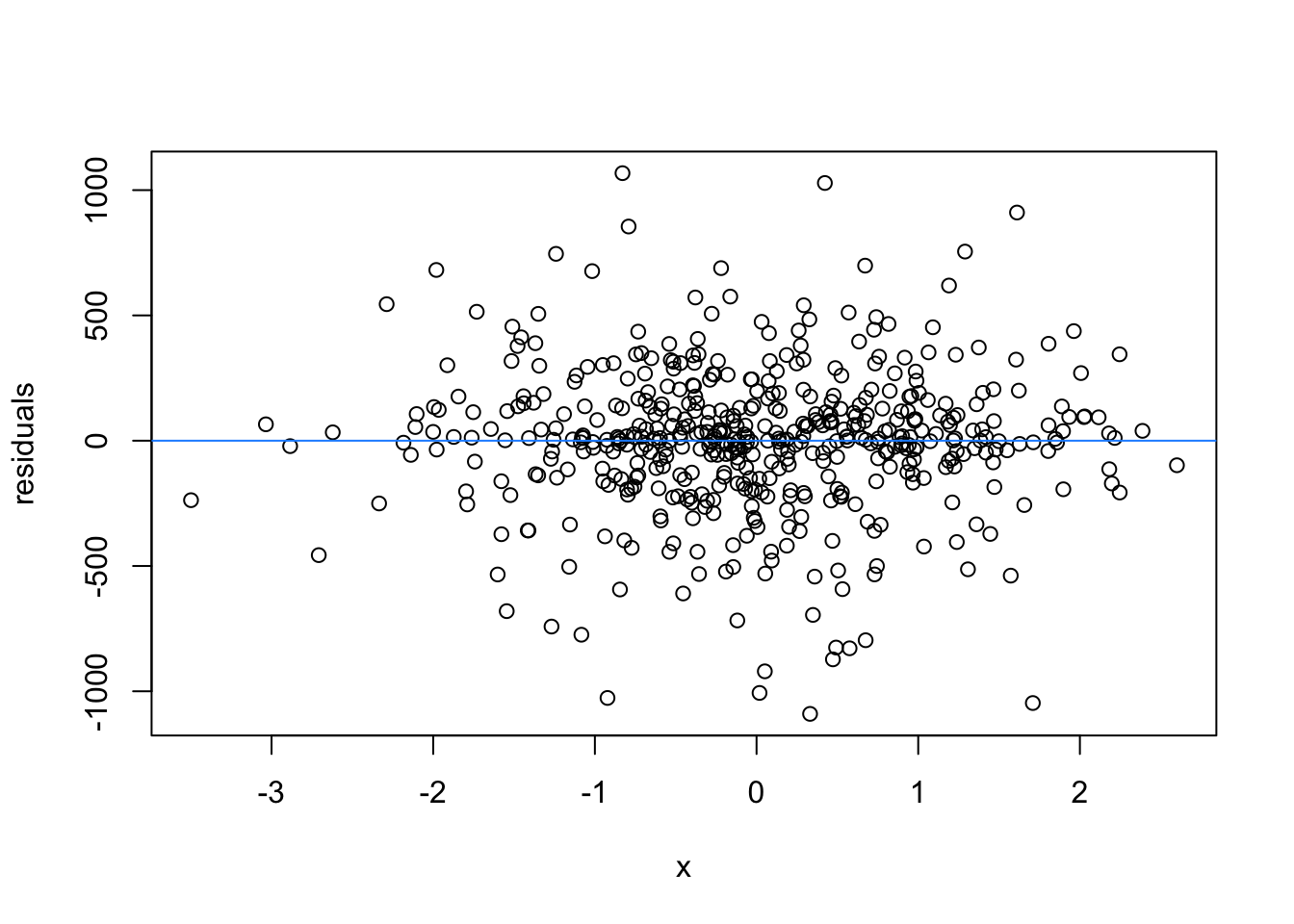
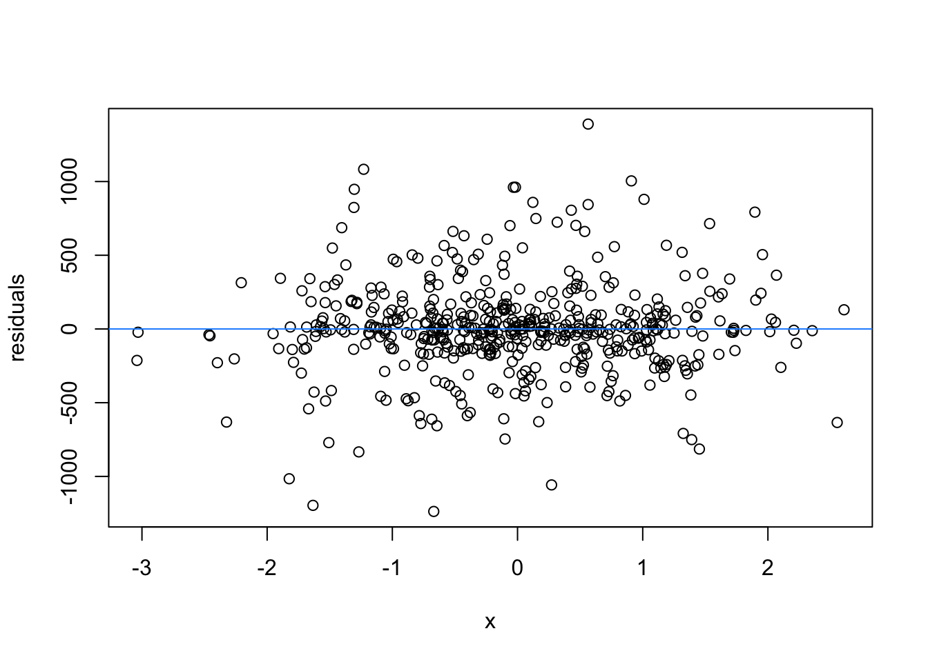
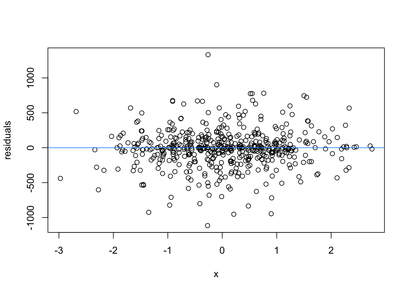
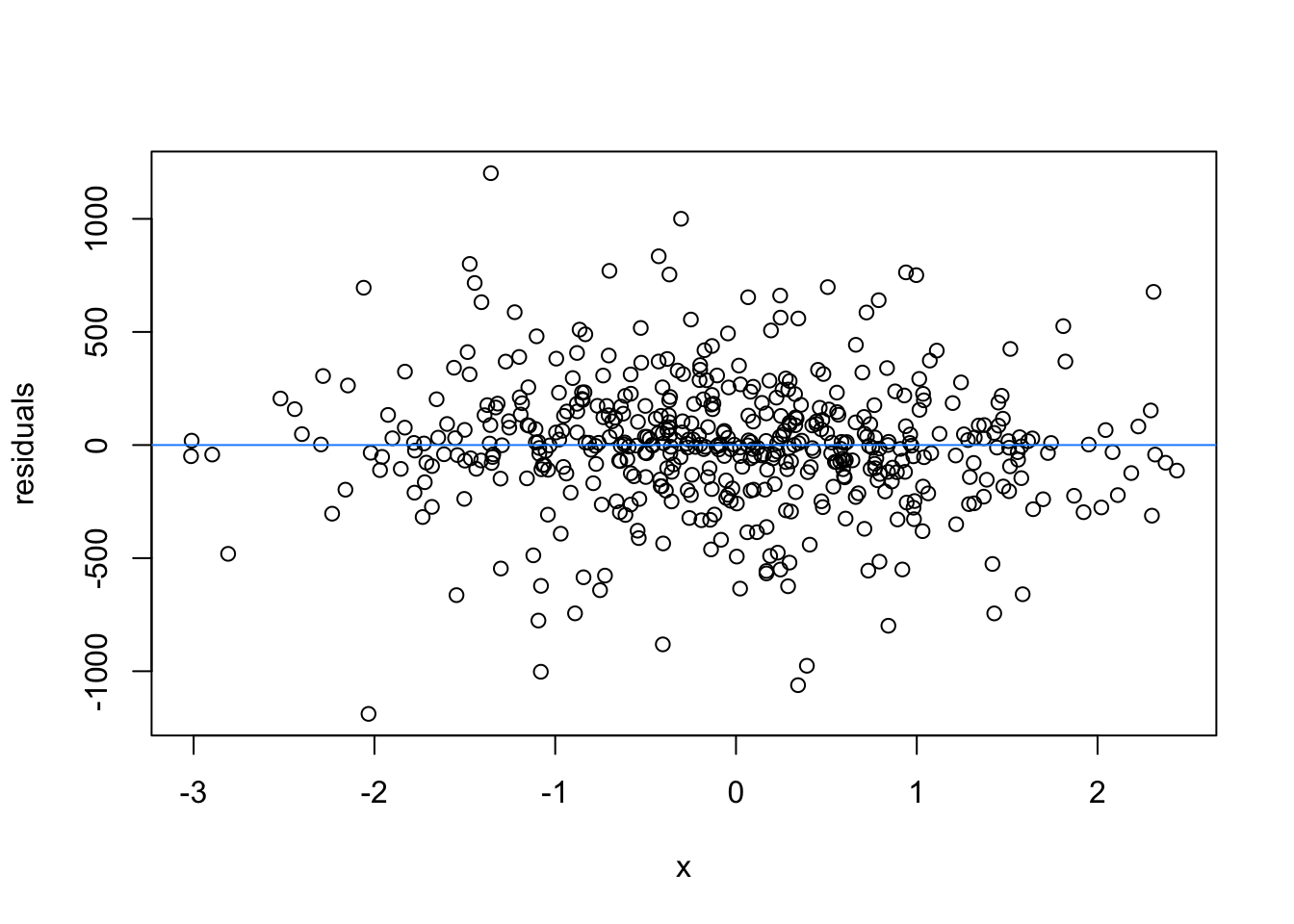
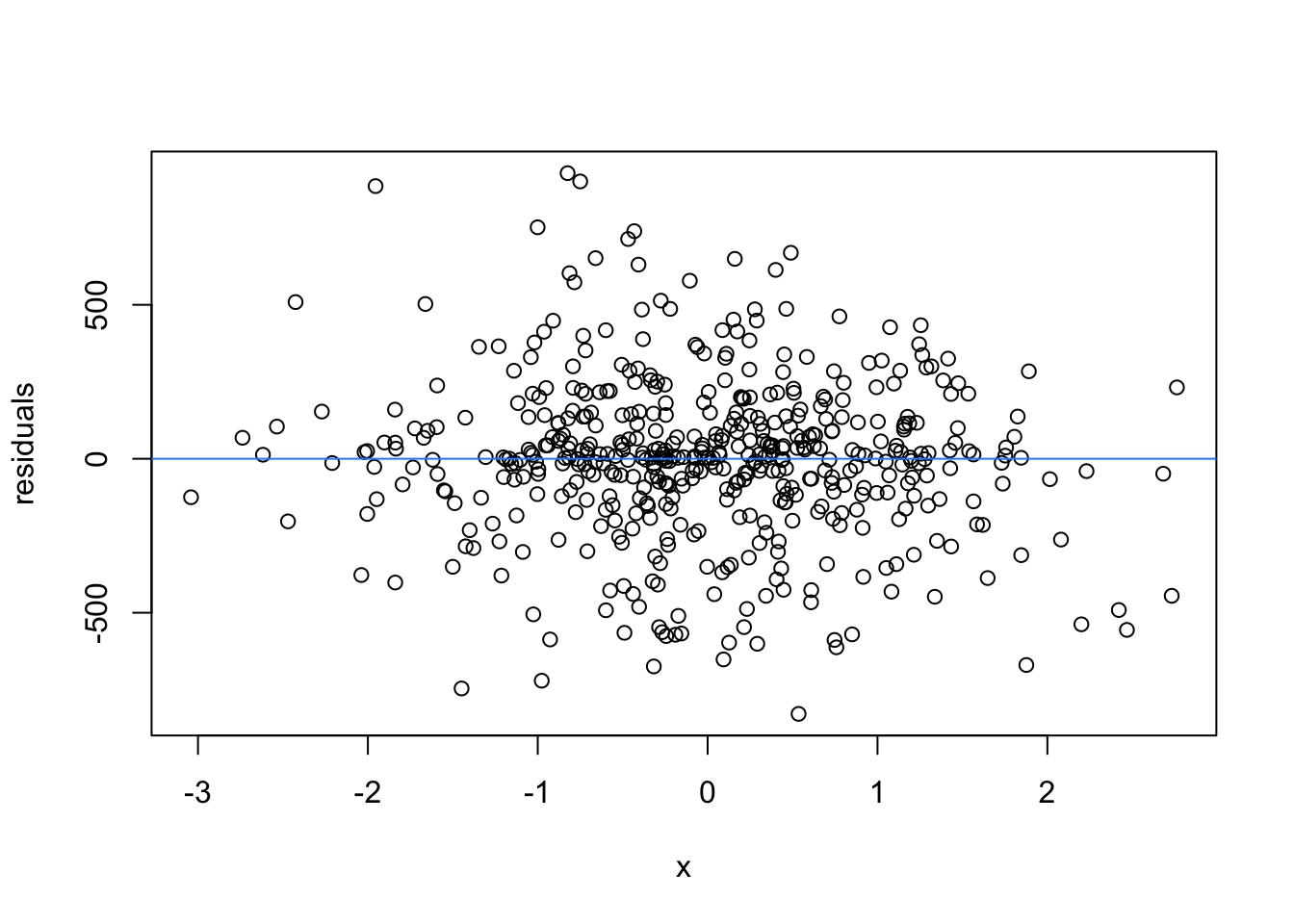
So lets image these are residuals and see what a good model looks like (assuming one predictor)
# this is for loop

# it says, for each value starting from 1 and ending at 9, repeat the following:

for(i in 1:9){
  set.seed(i)
  plot(rnorm(500), rnorm(500), xlab = 'x', ylab = 'residuals')
  abline(h = 0 , col = 'dodgerblue')
}
We can force heteroscedasticity into the simulated residuals - the simulated residuals are no longer a “blob”, but now take on the shape of a straight line
# this is for loop

# it says, for each value starting from 1 and ending at 9, repeat the following:

for(i in 1:9){
  set.seed(i)
  plot(rnorm(500), rnorm(500)*1:500, xlab = 'x', ylab = 'residuals')
  abline(h = 0, col = 'dodgerblue')
}
We normally have more than one predictor, right? So when we assess the residuals of these models, we assess homoscedasticity of the amalgamation of predictors. Let’s fit a model and look
library(tidyverse)── Attaching core tidyverse packages ──────────────────────── tidyverse 2.0.0 ──
✔ dplyr 1.1.4 ✔ readr 2.1.5
✔ forcats 1.0.1 ✔ stringr 1.5.2
✔ ggplot2 4.0.0 ✔ tibble 3.3.0
✔ lubridate 1.9.4 ✔ tidyr 1.3.1
✔ purrr 1.1.0
── Conflicts ────────────────────────────────────────── tidyverse_conflicts() ──
✖ dplyr::filter() masks stats::filter()
✖ dplyr::lag() masks stats::lag()
ℹ Use the conflicted package (<http://conflicted.r-lib.org/>) to force all conflicts to become errorsdat <- read_csv("winter_2017_iconicity.csv")Rows: 3001 Columns: 8
── Column specification ────────────────────────────────────────────────────────
Delimiter: ","
chr (2): Word, POS
dbl (6): SER, CorteseImag, Conc, Syst, Freq, Iconicity
ℹ Use `spec()` to retrieve the full column specification for this data.
ℹ Specify the column types or set `show_col_types = FALSE` to quiet this message.zscore all the variables (and log transform the frequency variable)
model_dat <- dat %>%
  mutate(SER_z = scale(SER),
         CorteseImag_z = scale(CorteseImag),
         Syst_z = scale(Syst),
         Freq_z = scale(log10(Freq)))
m1 <- lm(Iconicity ~ SER_z + CorteseImag_z + Syst_z + Freq_z, data = model_dat)
summary(m1)
Call:
lm(formula = Iconicity ~ SER_z + CorteseImag_z + Syst_z + Freq_z,
data = model_dat)
Residuals:
Min 1Q Median 3Q Max
-3.07601 -0.71411 -0.03824 0.67337 2.76066
Coefficients:
Estimate Std. Error t value Pr(>|t|)
(Intercept) 1.25694 0.03612 34.801 < 2e-16 ***
SER_z 0.51550 0.04160 12.391 < 2e-16 ***
CorteseImag_z -0.39364 0.03738 -10.531 < 2e-16 ***
Syst_z 0.04931 0.03229 1.527 0.127
Freq_z -0.26004 0.03867 -6.725 2.97e-11 ***
---
Signif. codes: 0 '***' 0.001 '**' 0.01 '*' 0.05 '.' 0.1 ' ' 1
Residual standard error: 1.002 on 984 degrees of freedom
(2012 observations deleted due to missingness)
Multiple R-squared: 0.2125, Adjusted R-squared: 0.2093
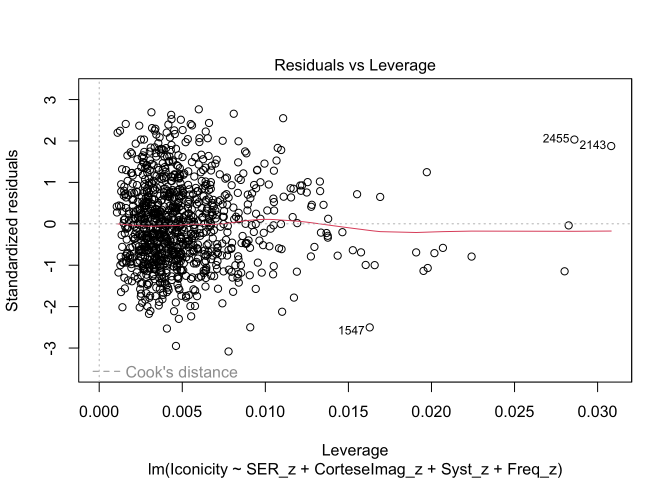
F-statistic: 66.36 on 4 and 984 DF, p-value: < 2.2e-16Check residuals:
plot(m1)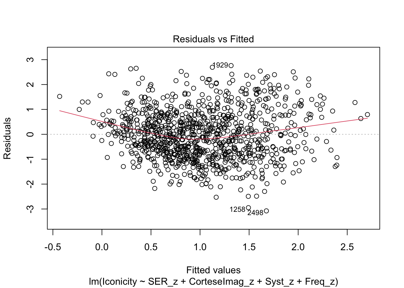
What are the added variable plot? They show us the effect of a predictor while all other predictors are accounted for, which allows us to test how residuals behave for one predictor (and thus assess their influence/fit).
See the excellent answer from silverfish here, who says:
“A lot of the value of an added variable plot comes at the regression diagnostic stage, especially since the residuals in the added variable plot are precisely the residuals from the original multiple regression.”
So what would we say about these variables? which are heteroscedastic, and which are homoscedastic.
car::avPlots(m1)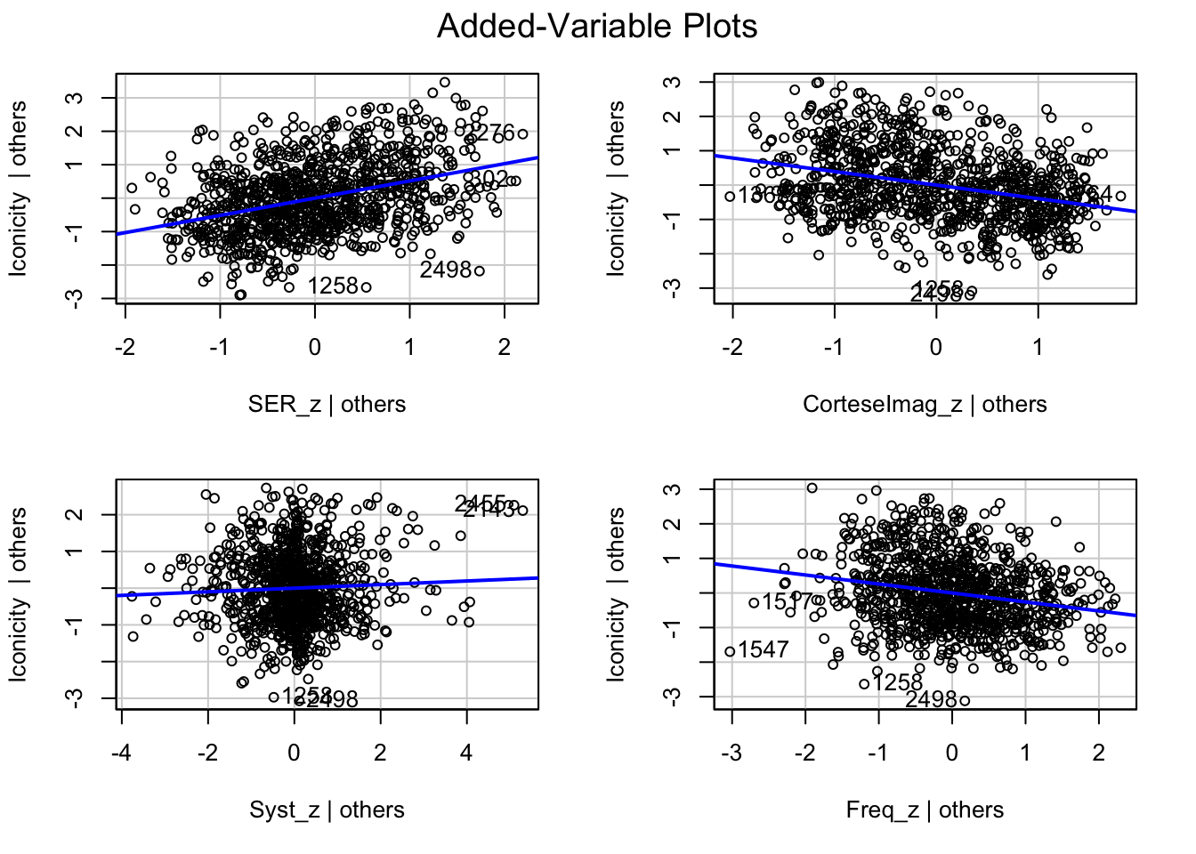
Collinearity is a property of two or more predictors being strongly correlated to the point that they (negatively) influence a model’s fit/behaviour. Why is this a problem? If two \(x\) variables are strongly correlated, they would have a similar effect on the \(y\) variable. By definition the multiple regression tries to determine how each predictor has an effect in the context of the other predictors. But if two predictors are doing the same thing, it is difficult to separate their individual effects. The book has an example with simulated data:
set.seed(42)
x <- rnorm(500)

y <- 10 + 3 * x + rnorm(500)
Look at the relationship between \(x\) and \(y\):
plot(x, y)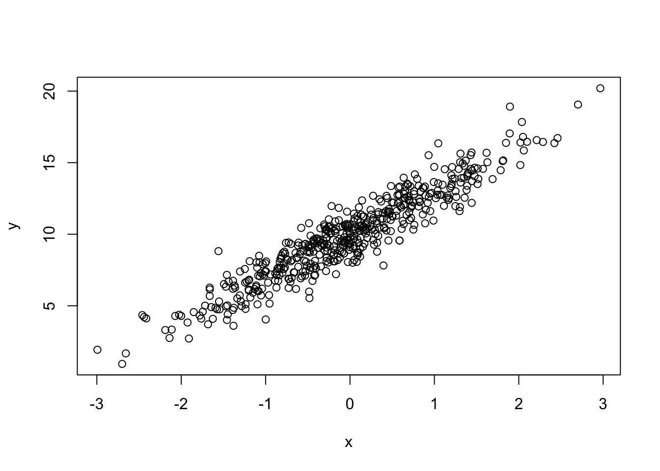
Now create an almost copy of \(x\), but vary it slightly by changinga few values only:
xx <- x
xx[500] <- x[250]
xx[499] <- -1
The new \(x\) has a similar relationship to \(y\)
plot(xx, y)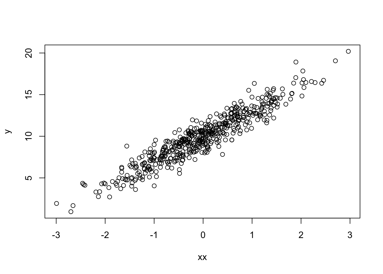
We can see the two \(x\) have an almost perfect relationship:
plot(xx, x)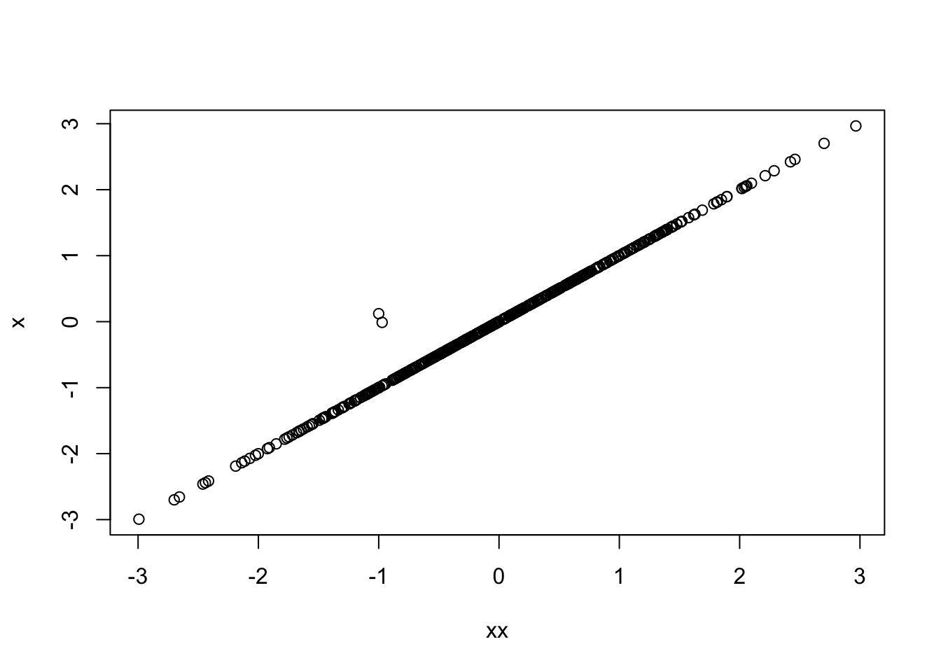
Marked by a strong positive correlation:
cor(xx, x)[1] 0.9977051What happens when they are put into a model together?
m2 <- lm(y ~ x + xx)We see that \(x\) has the predicted positive (and significant) effect, whereas \(xx\) is negative and not significant. The problem is that \(xx\) has nothing to contribute above and beyond the work that \(x\) already does (and \(x\) has a better fitting relation with \(y\))
summary(m2)
Call:
lm(formula = y ~ x + xx)
Residuals:
Min 1Q Median 3Q Max
-3.3501 -0.6623 0.0227 0.7338 3.5001
Coefficients:
Estimate Std. Error t value Pr(>|t|)
(Intercept) 9.98179 0.04633 215.461 < 2e-16 ***
x 2.11511 0.70275 3.010 0.00275 **
xx 0.87629 0.70142 1.249 0.21214
---
Signif. codes: 0 '***' 0.001 '**' 0.01 '*' 0.05 '.' 0.1 ' ' 1
Residual standard error: 1.033 on 497 degrees of freedom
Multiple R-squared: 0.8883, Adjusted R-squared: 0.8879
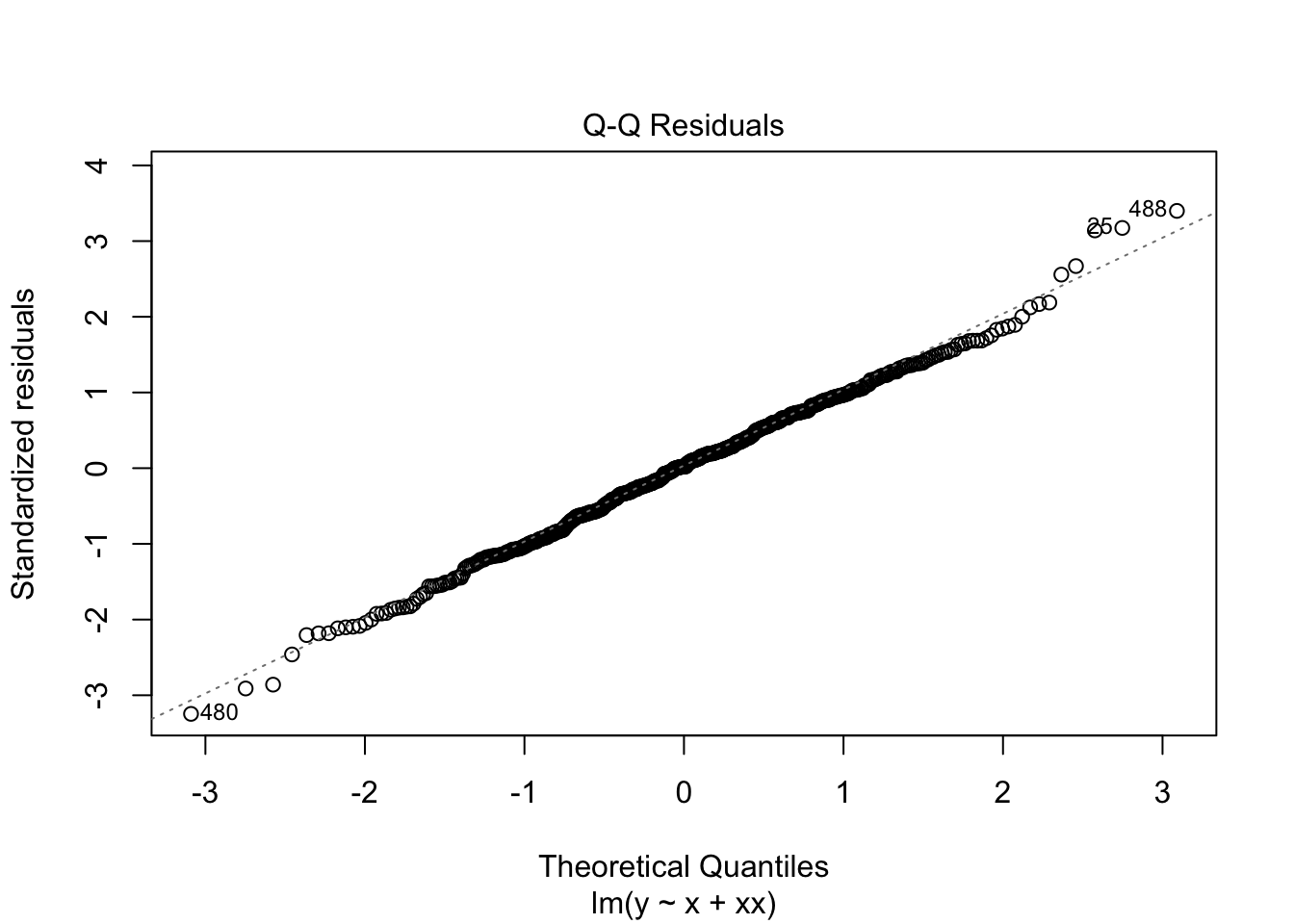
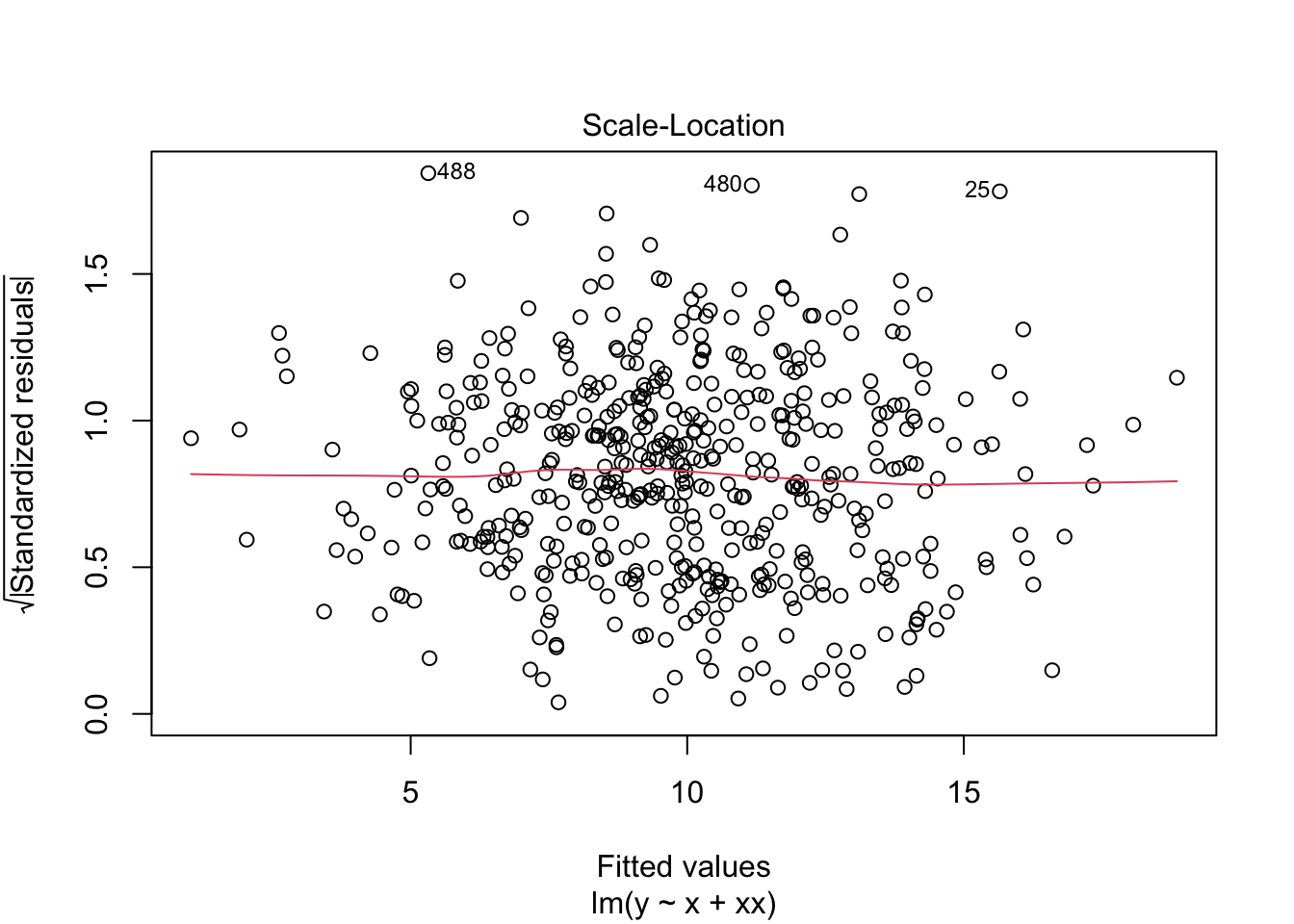
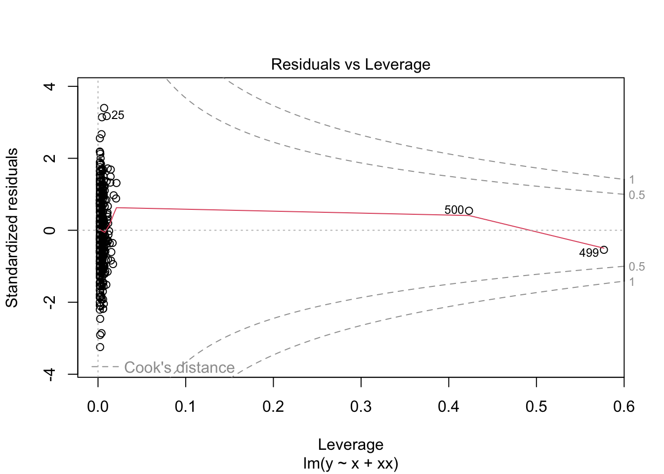
F-statistic: 1976 on 2 and 497 DF, p-value: < 2.2e-16What do the residuals look like?
plot(m2)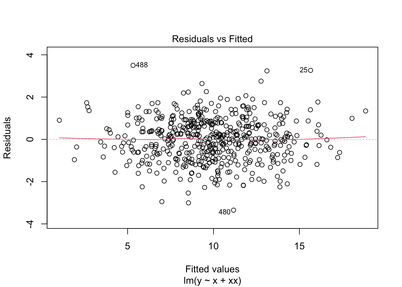
You can use the vif function from car:
car::vif(m2) x xx
218.1239 218.1239 However you might also be interested in the performance package which can do a host of model diagnostics:
performance::check_collinearity(m2)# Check for Multicollinearity
High Correlation
Term VIF VIF 95% CI adj. VIF Tolerance Tolerance 95% CI
x 218.12 [183.49, 259.33] 14.77 4.58e-03 [0.00, 0.01]
xx 218.12 [183.49, 259.33] 14.77 4.58e-03 [0.00, 0.01]performance::model_performance(m2)# Indices of model performance
AIC | AICc | BIC | R2 | R2 (adj.) | RMSE | Sigma
------------------------------------------------------------
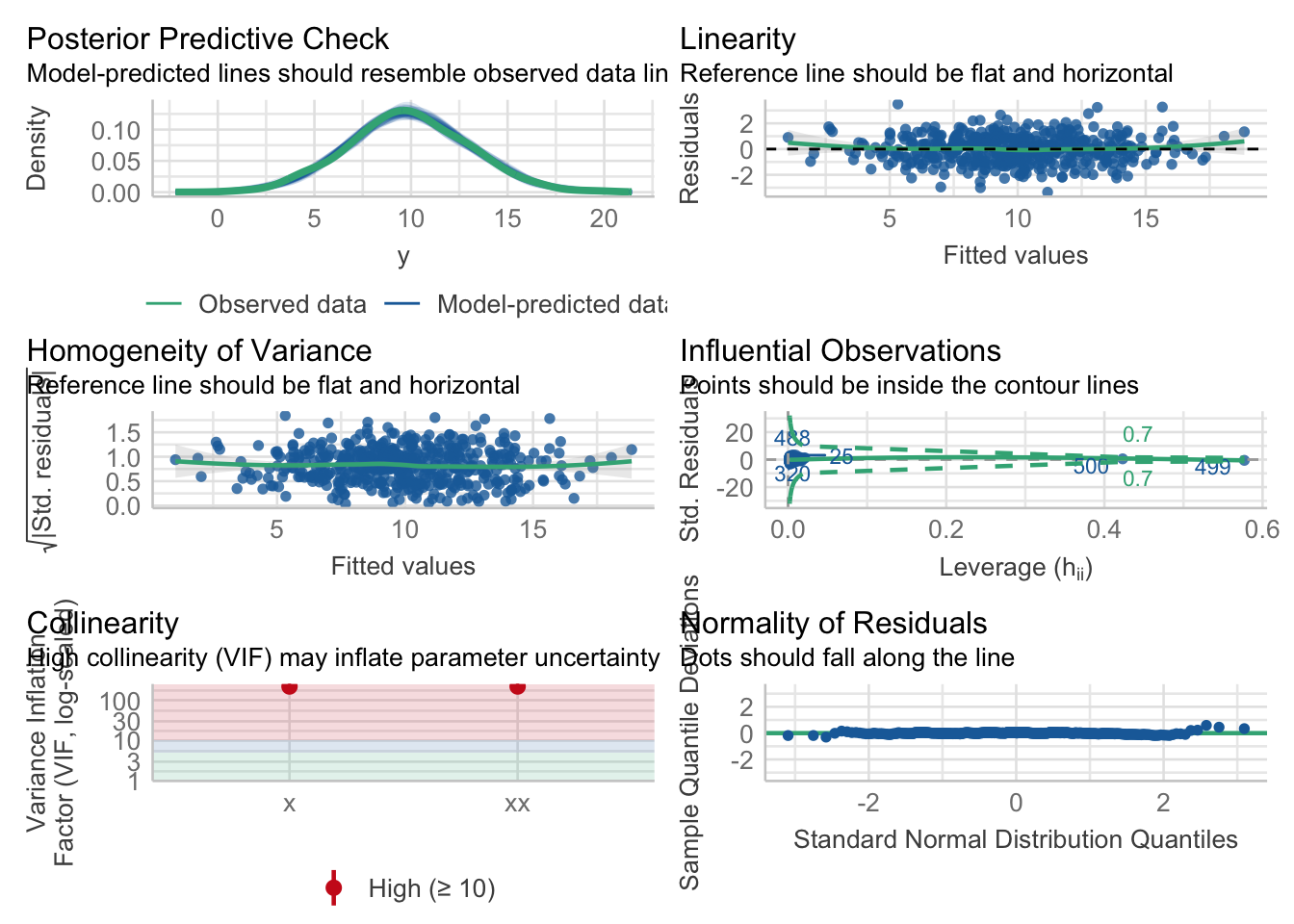
1456.7 | 1456.8 | 1473.6 | 0.888 | 0.888 | 1.030 | 1.033The check_model() function is a good one to get a broad overview of model diagnostics.
performance::check_model(m2)