library(tidyverse)
library(ggplot2)8.1-8.2
Chapter 8 - Interactions and Nonlinear Effects
8.1 Introduction
So far, we have discussed linear regression at its core: how one or more predictors can explain variations in a response variable.
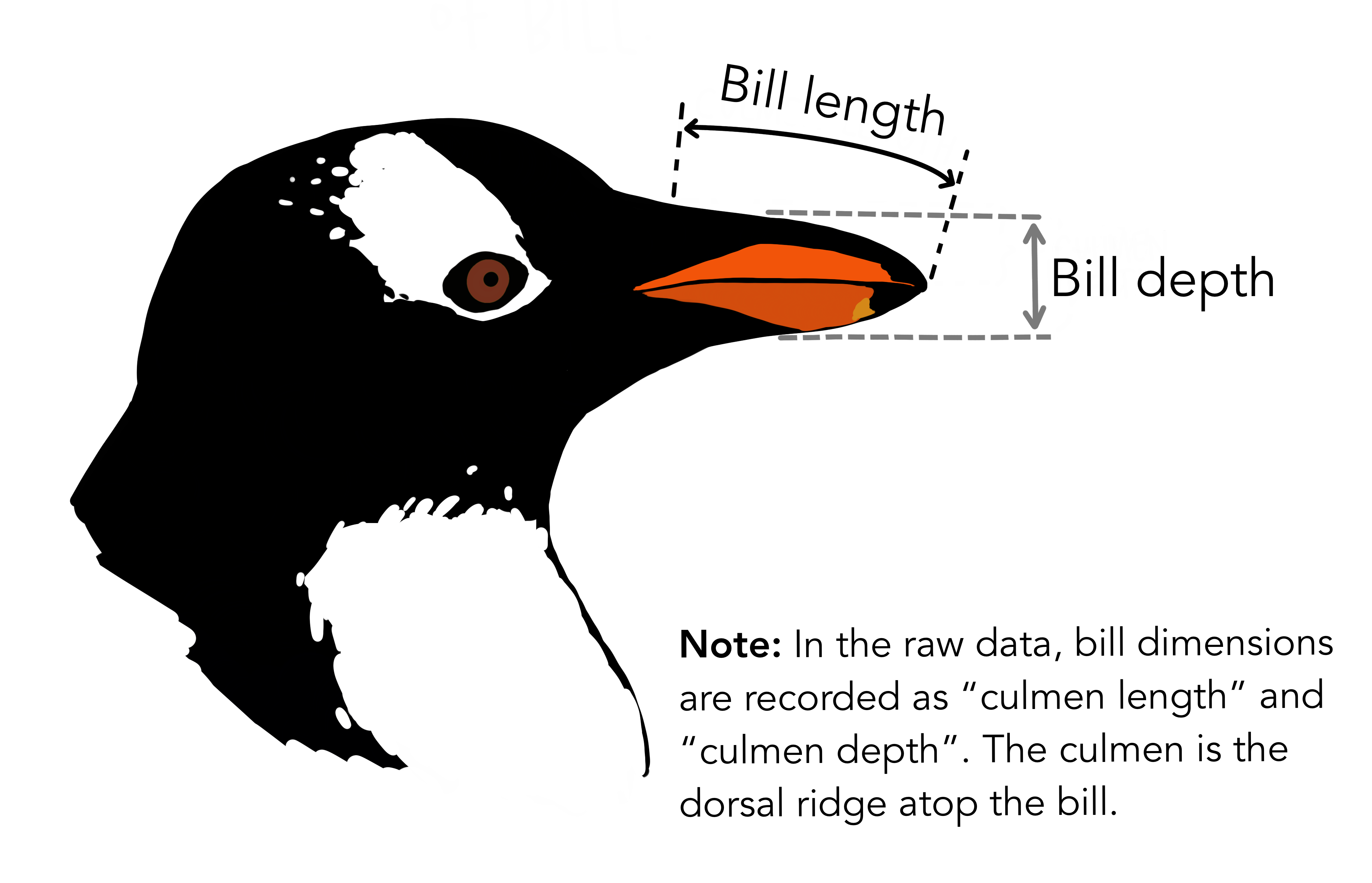
For example, using the penguins dataset from palmerpenguins library, we might be interested in how penguin’s bill length affects penguin’s body mass, put differently, how bill length can be used to predict body mass. (which explanation is more accurate?)
Similarly, in a wine quality dataset, we might examine the relationship between the percentage of alcohol (\(X\)) and the wine quality rating (\(Y\)).

However, the relationship is not always this simple. Predictors can depend on one another other, influencing each others relationship with a response variable. This idea is called an interaction.
For example, there is an interaction between penguin’s bill length and the bill depth. These two factors, together with its interaction, explains more variations in penguin’s body mass than the single predictos alone (although, it would be silly to think this is a causal relationship).
Equation for linear regression without an interaction:
\[ Y = \beta_0 + \beta_1 X_1 + \beta_2 X_2 + \epsilon \]
Equation for linear regression with an interaction:
\[ Y = \beta_0 + \beta_1 X_1 + \beta_2 X_2 + \beta_3 (X_1*X_2) + \epsilon \]
In Chapter 8, Winter discusses interactions between categorical x continuous variables, categorical x categorical variables, and continuous x continuous variables.
We will begin with the interaction between a categorical and a continuous variable.
8.2 Categorical x Continuous interactions
Bringing back an example dataset from Qi Yi’s week: iconicity (a resemblance between form and meaning)
icon <- read.csv("winter_2017_iconicity.csv")

head(icon)
Word POS SER CorteseImag Conc Syst Freq Iconicity
1 a Grammatical NA NA 1.46 NA 1041179 0.4615385
2 abide Verb NA NA 1.68 NA 138 0.2500000
3 able Adjective 1.73 NA 2.38 NA 8155 0.4666667
4 about Grammatical 1.20 NA 1.77 NA 185206 -0.1000000
5 above Grammatical 2.91 NA 3.33 NA 2493 1.0625000
6 abrasive Adjective NA NA 3.03 NA 23 1.3125000Variables of interest
Iconicity (Y - continuous) - rated from -5 to 5
Part-of-speech or POS (X - categorical) - 7 levels (Name, Interjection, Adverb, Grammatical, Adjective, Verb, Noun)
For today’s example, we will focus only on Noun and Verb.
- Sensory experience or SER (X - continuous) - derived from an existing dataset from a previous study that rated how strongly a word evokes a sensory experience (based on the five common sense), on a scale 1 to 7.
Now, we will filter only the data we are interested in.
icon_sel <- icon %>%
  select(1:3, 8) %>%
  filter(POS %in% c("Noun", "Verb"))

head(icon_sel)
Word POS SER Iconicity
1 abide Verb NA 0.2500000
2 academy Noun NA 0.6923077
3 accident Noun NA 1.3636364
4 accordion Noun NA -0.4545455
5 account Noun 2.30 -0.4285714
6 ache Noun 4.82 1.1538462There are many NA values in the SER column, as Qi Yi pointed out. However, we will (pretend) to ignore that issue.
Let’s briefly have a look at the data..
summary(icon_sel) Word POS SER Iconicity
Length:2261 Length:2261 Min. :1.000 Min. :-2.80000
Class :character Class :character 1st Qu.:2.550 1st Qu.: 0.09091
Mode :character Mode :character Median :3.270 Median : 0.70000
Mean :3.303 Mean : 0.85924
3rd Qu.:4.000 3rd Qu.: 1.50000
Max. :6.560 Max. : 4.46667
NA's :782 icon_sel %>% count(POS) POS n
1 Noun 1704
2 Verb 557If we are simply interested in the relationship between \(X\)s and \(Y\) without an interaction, we fit this model 1. These are referred to as main effects if they are not fit as an interaction.
model1 <- lm(Iconicity ~ SER + POS, data = icon_sel)

summary(model1)
Call:
lm(formula = Iconicity ~ SER + POS, data = icon_sel)

Residuals:
    Min      1Q  Median      3Q     Max
-3.0956 -0.7210 -0.1233  0.6146  3.6902

Coefficients:
            Estimate Std. Error t value Pr(>|t|)
(Intercept) -0.11935    0.10040  -1.189    0.235
SER          0.23319    0.02789   8.362   <2e-16 ***
POSVerb      0.60159    0.06388   9.418   <2e-16 ***
---
Signif. codes:  0 '***' 0.001 '**' 0.01 '*' 0.05 '.' 0.1 ' ' 1

Residual standard error: 1.045 on 1476 degrees of freedom
  (782 observations deleted due to missingness)
Multiple R-squared:  0.08226,   Adjusted R-squared:  0.08102
F-statistic: 66.15 on 2 and 1476 DF,  p-value: < 2.2e-16
“As always, you should spend considerable time interpreting the coefficients” – I’ll leave this to you :D
ggplot(icon_sel, aes(x = SER, y = Iconicity)) +
  geom_point(alpha = 0.5) +
  geom_smooth(method = lm) +
  labs(x = "sensory experience",
       y = "iconicity rating score",
       title = "Iconicity vs Sensory experience")+
  theme_bw()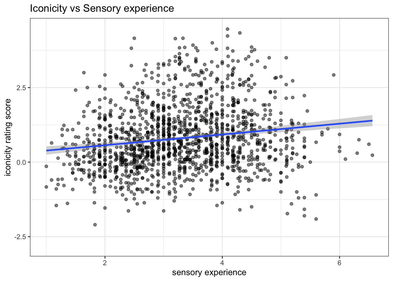
With this Model 1, the coefficient of each predictor is interpreted independently. For example, the SER coefficient indicates that for a 1-unit increase in SER, holding POS constant, the iconicity rating is predicted to increase by 0.23.
What does ‘holding POS constant’ mean?
It means that the effect of SER is estimated at the baseline. As long as POS is held as the baseline, the predicted change of 0.23 applies.
Now let’s look at this plot.
ggplot(icon_sel, aes(x = SER, y = Iconicity, color = POS)) +
  geom_point(size = 1.5, alpha = 0.5) +
  geom_smooth(method = "lm") +
  labs(x = "sensory experience",
       y = "iconicity rating score",
       title = "Iconicity vs Sensory experience across two POS",
       colour = "Part of speech")+
  theme_bw()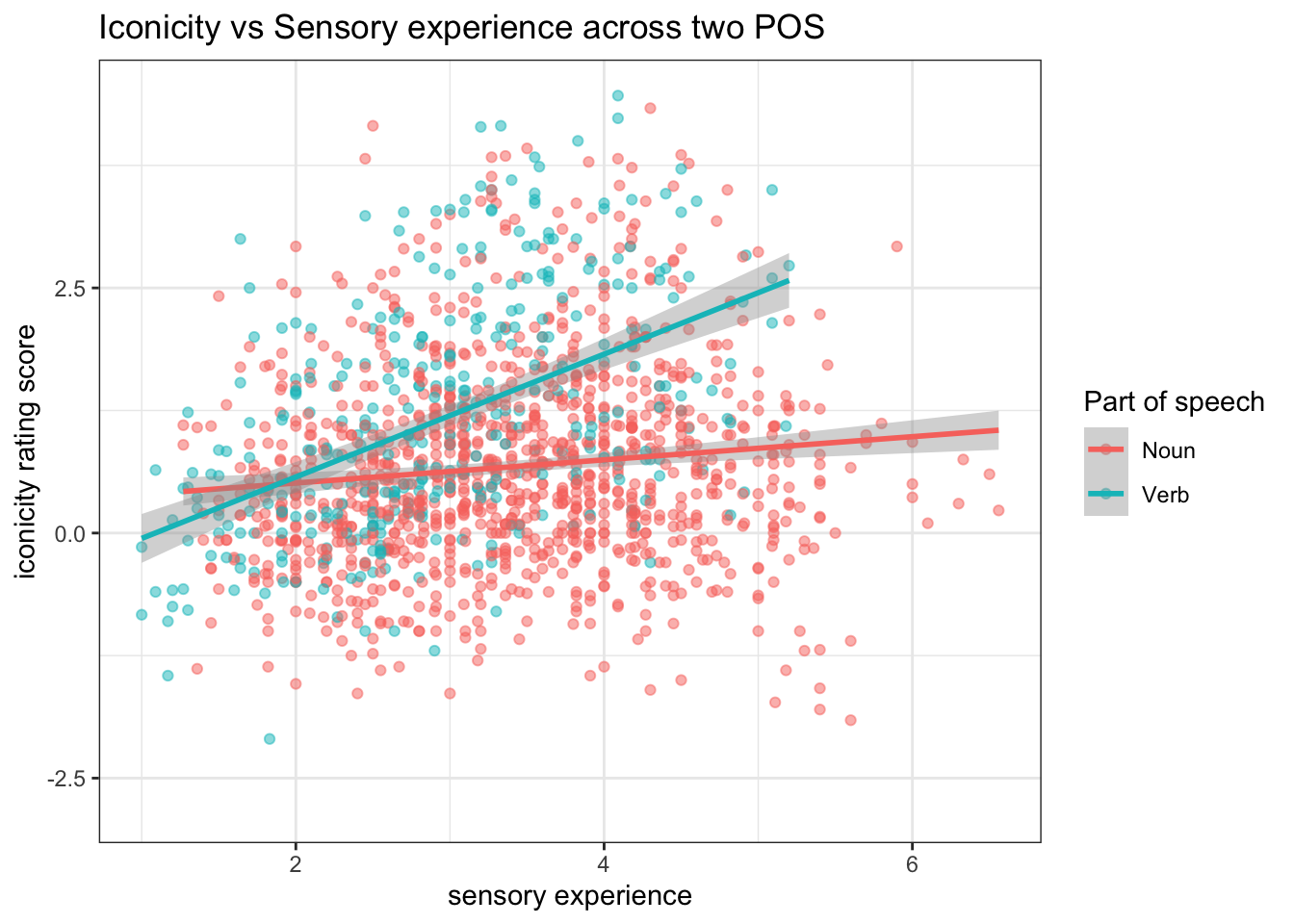
Question: What do these regression lines for Noun and Verb tell us?
The effect of SER on iconicity differs between nouns and verbs. Likewise, the degree to which nouns and verbs differ from each other in terms of iconicity also depends on what SER value one considers. This means that SER and POS are not independent in their effects. So, we should be careful about interpreting these predictors independently.
This brings us to… Multiple regression with an interaction model
model2 <- lm(Iconicity ~ SER * POS, data = icon_sel)

summary(model2)
Call:
lm(formula = Iconicity ~ SER * POS, data = icon_sel)

Residuals:
    Min      1Q  Median      3Q     Max
-2.8448 -0.7043 -0.1257  0.5864  3.5845

Coefficients:
            Estimate Std. Error t value Pr(>|t|)
(Intercept)  0.27394    0.11065   2.476  0.01341 *
SER          0.11817    0.03108   3.801  0.00015 ***
POSVerb     -0.95542    0.20971  -4.556 5.65e-06 ***
SER:POSVerb  0.50838    0.06535   7.780 1.36e-14 ***
---
Signif. codes:  0 '***' 0.001 '**' 0.01 '*' 0.05 '.' 0.1 ' ' 1

Residual standard error: 1.025 on 1475 degrees of freedom
  (782 observations deleted due to missingness)
Multiple R-squared:  0.1184,    Adjusted R-squared:  0.1166
F-statistic: 66.05 on 3 and 1475 DF,  p-value: < 2.2e-16
Interpreting coefficients
Intercept: When the SER = 0 and POS is held at nouns, the iconicity rating score is predicted to be 0.27.
SER coefficient: VERY IMPORTANT NOTE This is the coefficient only for nouns It means that, for nouns, a 1-unit increase in SER is predicted to increase iconicity by 0.12.
POSVerb coefficient: This coefficient is the difference between the predicted iconicity for noun and verb, when the word has SER = 0.
SER:POSVerb coefficient: This acts as a slope adjustment (think: what is being adjusted?). For verbs, the effect of SER on iconicity is adjusted by +0.51, meaning that the SER slope for verbs is higher than that of nouns by 0.51.
emmeans::joint_tests(model2) model term df1 df2 F.ratio p.value
SER 1 1475 129.872 <.0001
POS 1 1475 125.650 <.0001
SER:POS 1 1475 60.523 <.0001Centering continuous variable
In Model 2, we interpret the intercept and the POSVerb coefficient at SER = 0. However, in the data, SER was rated from 1 to 7. So, actually SER = 0 is arbitrary (and does not match reality).
ggplot(icon_sel, aes(x = SER, y = Iconicity, color = POS)) +
  geom_point(size = 1.5, alpha = 0.5) +
  geom_smooth(method = "lm", fullrange = TRUE) +
  labs(x = "sensory experience",
       y = "iconicity rating score",
       title = "Iconicity vs Sensory experience across two POS (Model 2)",
       colour = "Part of speech")+
  geom_vline(xintercept = 0, linetype = "dashed") +
  theme_bw()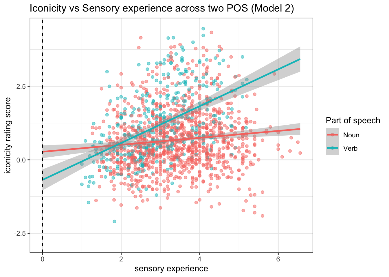
To facilitate interpretation, we should centre the continuous variable. “The interpretation for interaction for continuous variable is more comprehensible with the continuous variables are centered”.
icon_sel2 <- icon_sel %>% mutate(SER_c = scale(SER)) %>%
relocate(SER_c, .after = SER)summary(icon_sel2) Word POS SER
Length:2261 Length:2261 Min. :1.000
Class :character Class :character 1st Qu.:2.550
Mode :character Mode :character Median :3.270
Mean :3.303
3rd Qu.:4.000
Max. :6.560
NA's :782
SER_c.V1 Iconicity
Min. :-2.3144393573700 Min. :-2.80000
1st Qu.:-0.7566730383830 1st Qu.: 0.09091
Median :-0.0330654579519 Median : 0.70000
Mean : 0.0000000000000 Mean : 0.85924
3rd Qu.: 0.7005922277630 3rd Qu.: 1.50000
Max. : 3.2734191804100 Max. : 4.46667
NA's :782 Fit regression model again
model3 <- lm(Iconicity ~ SER_c * POS, data = icon_sel2)
summary(model3)
Call:
lm(formula = Iconicity ~ SER_c * POS, data = icon_sel2)

Residuals:
    Min      1Q  Median      3Q     Max
-2.8448 -0.7043 -0.1257  0.5864  3.5845

Coefficients:
              Estimate Std. Error t value Pr(>|t|)
(Intercept)    0.66423    0.03102  21.414  < 2e-16 ***
SER_c          0.11758    0.03093   3.801  0.00015 ***
POSVerb        0.72371    0.06456  11.209  < 2e-16 ***
SER_c:POSVerb  0.50585    0.06502   7.780 1.36e-14 ***
---
Signif. codes:  0 '***' 0.001 '**' 0.01 '*' 0.05 '.' 0.1 ' ' 1

Residual standard error: 1.025 on 1475 degrees of freedom
  (782 observations deleted due to missingness)
Multiple R-squared:  0.1184,    Adjusted R-squared:  0.1166
F-statistic: 66.05 on 3 and 1475 DF,  p-value: < 2.2e-16
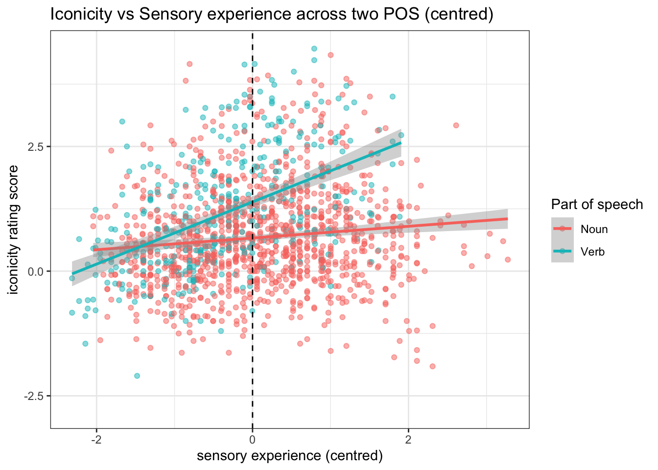
Now, how do you interpret the coefficients?
In particular, look at POSVerb coefficient!
ggplot(icon_sel2, aes(x = SER_c, y = Iconicity, color = POS)) +
  geom_point(size = 1.5, alpha = 0.5) +
  geom_smooth(method = "lm") +
  labs(x = "sensory experience (centred)",
             y = "iconicity rating score",
             title = "Iconicity vs Sensory experience across two POS (centred)",
        colour = "Part of speech")+
  geom_vline(xintercept = 0, linetype = "dashed")+
  theme_bw()