# equals 2*2
2^2
[1] 4Section 5.4
“Positive skew is ubiquitous in linguistic data.” p. 90
# equals 2*2
2^2[1] 4# equals 2*2*2*2*2*2*2*2*2*2
2^10[1] 1024The base exp() function in R will use the constant of 2.71828 known as \({e}\) or Euler’s number and raise it to whatever power you give it:
exp(43)[1] 4.727839e+18Verify manually:
2.71828^43[1] 4.727703e+18The base log() function in R does the same thing, but in reverse. This is called the natural logarithm
log(2.71828^43)[1] 42.99997One thing to note is that with log() is that if we log() a 0, the result is Inf
log(0)[1] -InfWe can instead use log1p() to avoid this, if our data have zeroes. This function adds 1 to all values before computing the log. (bonus - what kind of transformation is adding 1 to all values?)
log1p(0)[1] 0“The logarithm takes large numbers and shrinks them. The exponential function takes small numbers and grows them.” p. 91
The logarithm of a larger number is more extreme then a smaller number. Compare how much reduction occurs in these two examples:
log(10)[1] 2.302585log(1000)[1] 6.907755Bodo Winter recommends log10() because it:
log10(10)[1] 1log10(1000)[1] 3One thing that a log transformation can help with is skewed data. Skewed data is usually marked by a long tail, which means that a relatively smaller number of data points are extended to one direction of a distribution.
Let’s look at data from my L2 ELP project.
library(tidyverse)── Attaching core tidyverse packages ──────────────────────── tidyverse 2.0.0 ──
✔ dplyr 1.1.4 ✔ readr 2.1.5
✔ forcats 1.0.1 ✔ stringr 1.5.2
✔ ggplot2 4.0.0 ✔ tibble 3.3.0
✔ lubridate 1.9.4 ✔ tidyr 1.3.1
✔ purrr 1.1.0
── Conflicts ────────────────────────────────────────── tidyverse_conflicts() ──
✖ dplyr::filter() masks stats::filter()
✖ dplyr::lag() masks stats::lag()
ℹ Use the conflicted package (<http://conflicted.r-lib.org/>) to force all conflicts to become errorsdat <- read_csv('L2_ELP.csv')Rows: 3318 Columns: 4
── Column specification ────────────────────────────────────────────────────────
Delimiter: ","
chr (1): word
dbl (3): RT, logWF, length
ℹ Use `spec()` to retrieve the full column specification for this data.
ℹ Specify the column types or set `show_col_types = FALSE` to quiet this message.This data has been pre-trimmed, meaning that very extreme values were already removed. Here we see some mild skewness in the histgram:
ggplot(dat, aes(x = RT)) +
  geom_histogram(binwidth = 10, fill = 'dodgerblue', alpha = .5)
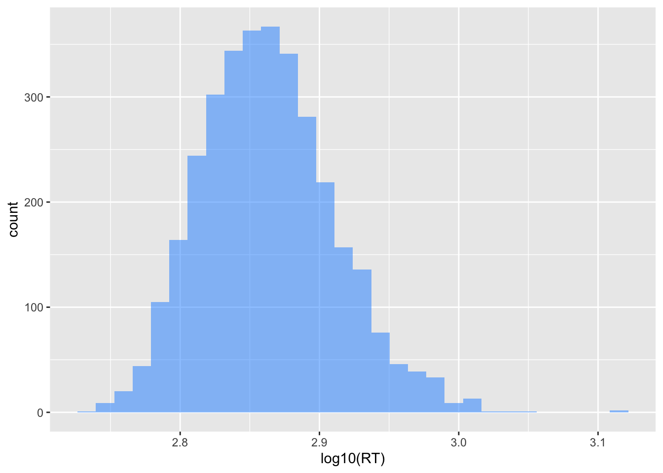
ggplot(dat, aes(x = log10(RT))) +
  geom_histogram(fill = 'dodgerblue', alpha = .5)
`stat_bin()` using `bins = 30`. Pick better value `binwidth`.
Compare the x-axis and the distributions of the two plots. Do you see how the logarithmic transformation has “shrunk” the gaps between the raw values?
For example, the value that was at 1300 is now near 3.2.
…“it’s worth noting that many cognitive and linguistic phenomena are scaled logarithmically.” p. 94
m1 <- lm(RT ~ logWF, data = dat)m2 <- lm(log10(RT) ~ logWF, data = dat)plot(density(resid(m1)))
plot(density(resid(m2)))