── Attaching core tidyverse packages ──────────────────────── tidyverse 2.0.0 ──
✔ dplyr     1.1.4     ✔ readr     2.1.5
✔ forcats   1.0.1     ✔ stringr   1.5.2
✔ ggplot2   4.0.0     ✔ tibble    3.3.0
✔ lubridate 1.9.4     ✔ tidyr     1.3.1
✔ purrr     1.1.0
── Conflicts ────────────────────────────────────────── tidyverse_conflicts() ──
✖ dplyr::filter() masks stats::filter()
✖ dplyr::lag()    masks stats::lag()
ℹ Use the conflicted package (<http://conflicted.r-lib.org/>) to force all conflicts to become errors
library(palmerpenguins)
Attaching package: 'palmerpenguins'

The following objects are masked from 'package:datasets':

    penguins, penguins_raw
data(penguins)
Significance in multiple regression
What does it mean for a single predictor to be “significant” in the context of a multiple regression? Well, it means that the model has taken in information from more than one independent variable. Sometimes this is described as “controlling” for other variables. But what is more interesting to us here is that the significance values will change in the presense of other variables. We can use penguins to demonstrate.
# load in data and z-score some variables. penguins_lm <- penguins %>%drop_na() %>%mutate(bl_c =scale(bill_length_mm), bd_c =scale(bill_depth_mm), flipper_c =scale(flipper_length_mm))
As always, we are interested in predicting the body mass of penguins.
If we fit a model with all 3 variables, we get a significant effect of flipper length, whereas bill length and bill depth are not significant.
Call:
lm(formula = body_mass_g ~ bl_c + bd_c + flipper_c, data = penguins_lm)

Residuals:
     Min       1Q   Median       3Q      Max
-1051.37  -284.50   -20.37   241.03  1283.51

Coefficients:
            Estimate Std. Error t value Pr(>|t|)
(Intercept)  4207.06      21.54 195.345   <2e-16 ***
bl_c           18.01      29.34   0.614    0.540
bd_c           35.12      27.23   1.290    0.198
flipper_c     711.47      35.00  20.327   <2e-16 ***
---
Signif. codes:  0 '***' 0.001 '**' 0.01 '*' 0.05 '.' 0.1 ' ' 1

Residual standard error: 393 on 329 degrees of freedom
Multiple R-squared:  0.7639,    Adjusted R-squared:  0.7618
F-statistic: 354.9 on 3 and 329 DF,  p-value: < 2.2e-16
Caution
So, what does it mean for flipper length to be significant in this context?
It means that not only is flipper length significant, it remains significant even when the model has information about other predictors. When taking into account the effects of bill length and bill depth, variation in flipper length is still an important variable. And, conversely, bill length and bill depth are not significant in light of information about flipper length.
Does this mean that bill length and bill depth are not significant? Well, it depends. Look at the following 3 models:
m2 <-lm(body_mass_g ~ bl_c, data = penguins_lm)summary(m2)
Call:
lm(formula = body_mass_g ~ bl_c, data = penguins_lm)

Residuals:
     Min       1Q   Median       3Q      Max
-1759.38  -468.82    27.79   464.20  1641.00

Coefficients:
            Estimate Std. Error t value Pr(>|t|)
(Intercept)  4207.06      35.70  117.85   <2e-16 ***
bl_c          474.64      35.75   13.28   <2e-16 ***
---
Signif. codes:  0 '***' 0.001 '**' 0.01 '*' 0.05 '.' 0.1 ' ' 1

Residual standard error: 651.4 on 331 degrees of freedom
Multiple R-squared:  0.3475,    Adjusted R-squared:  0.3455
F-statistic: 176.2 on 1 and 331 DF,  p-value: < 2.2e-16
m3 <-lm(body_mass_g ~ bd_c, data = penguins_lm)summary(m3)
Call:
lm(formula = body_mass_g ~ bd_c, data = penguins_lm)

Residuals:
     Min       1Q   Median       3Q      Max
-1616.08  -510.38   -68.67   486.51  1811.12

Coefficients:
            Estimate Std. Error t value Pr(>|t|)
(Intercept)  4207.06      38.96 107.986   <2e-16 ***
bd_c         -380.07      39.02  -9.741   <2e-16 ***
---
Signif. codes:  0 '***' 0.001 '**' 0.01 '*' 0.05 '.' 0.1 ' ' 1

Residual standard error: 710.9 on 331 degrees of freedom
Multiple R-squared:  0.2228,    Adjusted R-squared:  0.2205
F-statistic: 94.89 on 1 and 331 DF,  p-value: < 2.2e-16
m4 <-lm(body_mass_g ~ bl_c + bd_c, data = penguins_lm)summary(m4)
Call:
lm(formula = body_mass_g ~ bl_c + bd_c, data = penguins_lm)

Residuals:
     Min       1Q   Median       3Q      Max
-1806.74  -456.82    15.33   471.07  1541.34

Coefficients:
            Estimate Std. Error t value Pr(>|t|)
(Intercept)  4207.06      32.30 130.257  < 2e-16 ***
bl_c          409.13      33.23  12.313  < 2e-16 ***
bd_c         -286.54      33.23  -8.624 2.76e-16 ***
---
Signif. codes:  0 '***' 0.001 '**' 0.01 '*' 0.05 '.' 0.1 ' ' 1

Residual standard error: 589.4 on 330 degrees of freedom
Multiple R-squared:  0.4675,    Adjusted R-squared:  0.4642
F-statistic: 144.8 on 2 and 330 DF,  p-value: < 2.2e-16
Each model shows significant effects for bill length and bill depth, even when both are combined into a single model. So it is not the case that they do not have a significant relationship, it’s just that when we put them into a model with flipper length, this relationship becomes redundant or less important when compared to flipper length.
Multicollinearity?
This probably means that the variables are all inherently capturing some similar property of the penguins (i.e., body size), and are likely correlated.
We see that they are correlated, with relatively strong correlation between flipper length and both bill measures. They do not perfectly co vary, so they are capturing overlap as well as their own variation in penguins, but it seems in this case flipper length might make information about the length and depth of bills redundant.
Using VIF to check multicollinearity
Another (and probably better) way to check for redundancy and overlap among your predictors is to use variance inflation factor (VIF), which tests for overlap in the context of the fit model. Unlike a correlation matrix, which only captures pairwise relationships between predictors, VIF accounts for the combined overlap of all predictors simultaneously — making it better at detecting multicollinearity that only emerges when multiple variables are considered together.
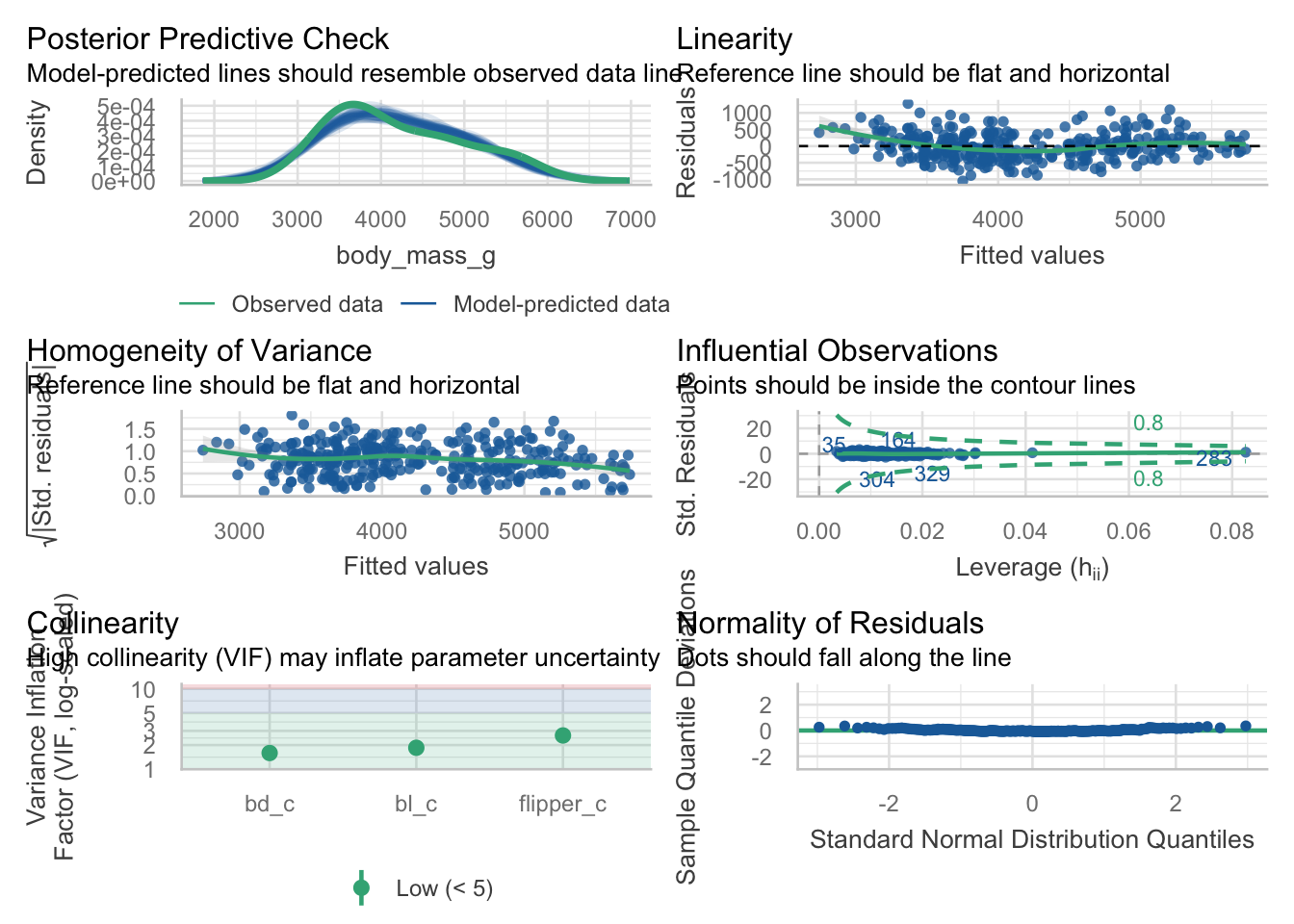
We can use the check_collinearity function from the wonderful performance package to test a fit model. Here we see that actually, our variables are not very strongly correlated and that the full model does not really suffer from multicollinearity.
May as well get the whole model check while we are at it? Note that VIF is one of the bits of information provided.
check_model(m1)
Some of the variables were in matrix-format - probably you used
  `scale()` on your data?
  If so, and you get an error, please try `datawizard::standardize()` to
  standardize your data.
Some of the variables were in matrix-format - probably you used
  `scale()` on your data?
  If so, and you get an error, please try `datawizard::standardize()` to
  standardize your data.
So what?
We need to understand that putting variables into a multiple regression will impact other variables, even when they are not in an interaction
This can lead to several problems - too many similar variables might make something look “not significant”, and not including the right variables may inflate the importance of other variables.
The idea of “controlling” for variables simply means including them in the model. It is a conceptual difference whether a variable is a “control” variable or whether it is an independent variable related to your hypotheses.
Confidence intervals
p-values should not be the only thing we care about - we want measures of effect sizes plus precision of our estimates.
The standard error from the model output gives us precision as it relates to the point estimate:
summary(m1)
Call:
lm(formula = body_mass_g ~ bl_c + bd_c + flipper_c, data = penguins_lm)

Residuals:
     Min       1Q   Median       3Q      Max
-1051.37  -284.50   -20.37   241.03  1283.51

Coefficients:
            Estimate Std. Error t value Pr(>|t|)
(Intercept)  4207.06      21.54 195.345   <2e-16 ***
bl_c           18.01      29.34   0.614    0.540
bd_c           35.12      27.23   1.290    0.198
flipper_c     711.47      35.00  20.327   <2e-16 ***
---
Signif. codes:  0 '***' 0.001 '**' 0.01 '*' 0.05 '.' 0.1 ' ' 1

Residual standard error: 393 on 329 degrees of freedom
Multiple R-squared:  0.7639,    Adjusted R-squared:  0.7618
F-statistic: 354.9 on 3 and 329 DF,  p-value: < 2.2e-16
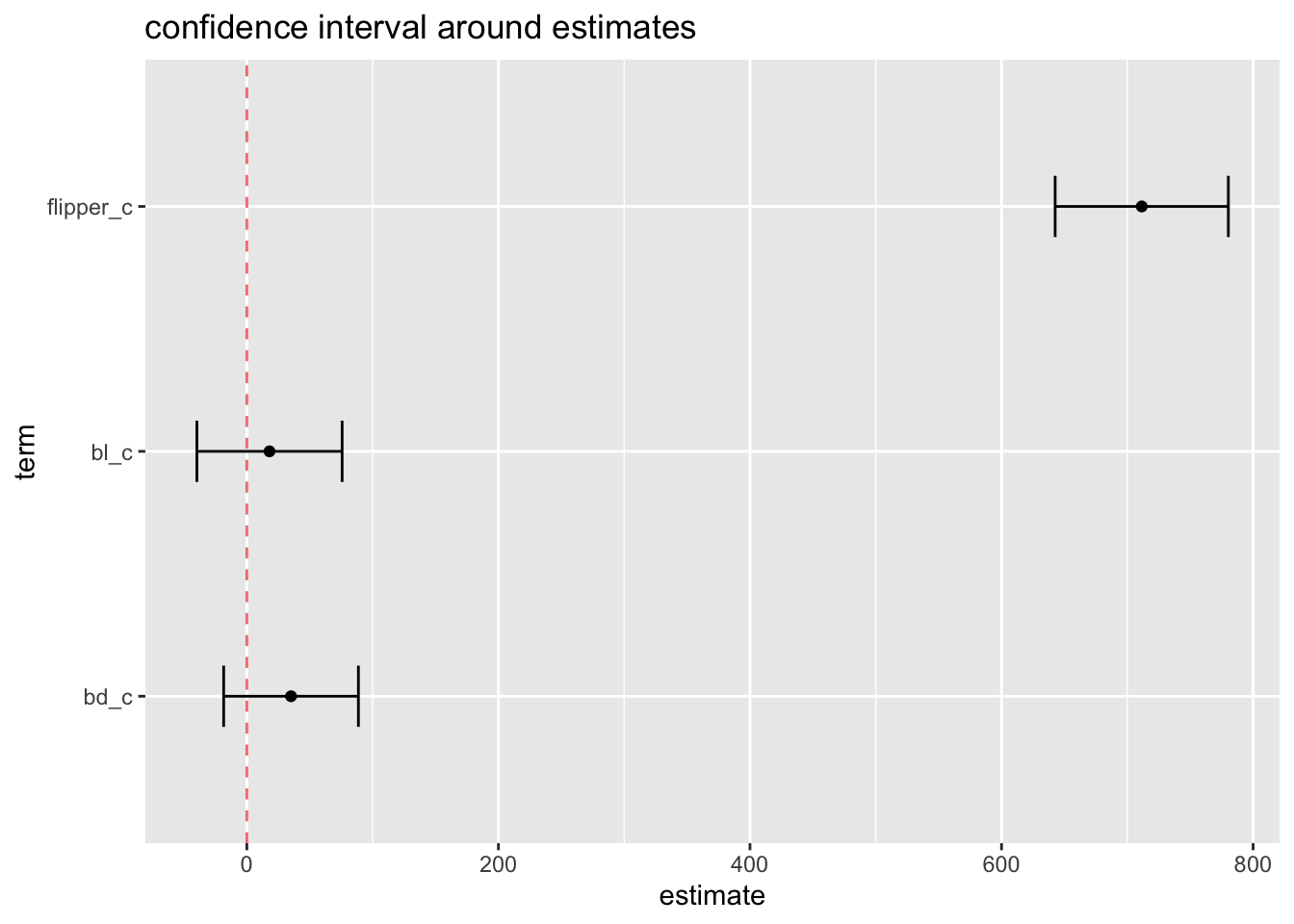
m1_plot_ci <-cbind(tidy(m1),as.data.frame(confint(m1)))[2:4,]ggplot(m1_plot_ci, aes(x = estimate, y = term)) +geom_point() +geom_errorbar(aes(xmin =`2.5 %`, xmax =`97.5 %`), width = .25) +labs(title ='confidence interval around estimates') +geom_vline(xintercept =0, color ='lightcoral', lty ='dashed')
Important
Standard error: precision of estimate, function of sample size and standard deviation Confidence interval: Over the long run, 95% of your confidence intervals will contain the true population parameter. (Yes this is annoyingly precise and somewhat counter intuitive).
So we can read this to say that more often than not we capture the true parameter. Just like p-values, more often than not, we are not making a type I error.
Quickly look at an interaction
Let’s complicate this with a continuous by categorical interaction.
What is significant here?
m5 <-lm(body_mass_g ~ species * flipper_c, data = penguins_lm)summary(m5)
Call:
lm(formula = body_mass_g ~ species * flipper_c, data = penguins_lm)

Residuals:
    Min      1Q  Median      3Q     Max
-900.90 -247.01  -25.53  197.19 1143.33

Coefficients:
                           Estimate Std. Error t value Pr(>|t|)
(Intercept)                 4061.30      59.40  68.377  < 2e-16 ***
speciesChinstrap            -150.39      81.11  -1.854  0.06460 .
speciesGentoo                149.95     108.12   1.387  0.16641
flipper_c                    458.16      65.76   6.967 1.78e-11 ***
speciesChinstrap:flipper_c    26.41     110.22   0.240  0.81077
speciesGentoo:flipper_c      301.01      97.65   3.083  0.00223 **
---
Signif. codes:  0 '***' 0.001 '**' 0.01 '*' 0.05 '.' 0.1 ' ' 1

Residual standard error: 368.4 on 327 degrees of freedom
Multiple R-squared:  0.7938,    Adjusted R-squared:  0.7906
F-statistic: 251.7 on 5 and 327 DF,  p-value: < 2.2e-16
packages like emmeans make this far easier to check
library(emmeans)
Welcome to emmeans.
Caution: You lose important information if you filter this package's results.
See '? untidy'
What do you notice about this output? What value is flipper length set to?
emmeans(m5, pairwise ~ species | flipper_c)
$emmeans
flipper_c = 3.5e-16:
 species   emmean   SE  df lower.CL upper.CL
 Adelie      4061 59.4 327     3944     4178
 Chinstrap   3911 55.2 327     3802     4020
 Gentoo      4211 90.3 327     4034     4389

Confidence level used: 0.95

$contrasts
flipper_c = 3.5e-16:
 contrast           estimate    SE  df t.ratio p.value
 Adelie - Chinstrap      150  81.1 327   1.854  0.1539
 Adelie - Gentoo        -150 108.0 327  -1.387  0.3489
 Chinstrap - Gentoo     -300 106.0 327  -2.836  0.0134

P value adjustment: tukey method for comparing a family of 3 estimates
Pick a point, or, regions of significance
Examine the species pairwise comparisons at different levels of flipper length. Since I have z-scored the variable, I can set the range to be +/-2 standard deviations, as well as the mean very easily:
# call just the contrasts, for spaceemmeans(m5, pairwise ~ species | flipper_c, at =list(flipper_c =c(-2,-1,0,1,2)))$contrasts
What did you notice about the pairwise comparisons? What is going on here?
We can sort of see this with a plot using emmip from emmeans:
emmip(m5, ~ species|flipper_c, var ='flipper_c', at =list(flipper_c =c(-2,-1,0,1,2)))
Warning: `aes_()` was deprecated in ggplot2 3.0.0.
ℹ Please use tidy evaluation idioms with `aes()`
ℹ The deprecated feature was likely used in the emmeans package.
  Please report the issue at <https://github.com/rvlenth/emmeans/issues>.
Let’s build a more robust plot. First save the emmip to an object, ask for CIs, and ask NOT to plot it yet.
m5_plot <-emmip(m5, ~ species|flipper_c, var ='flipper_c', at =list(flipper_c =c(-2,-1,0,1,2)),plotit = F,CIs = T )
Here is a plot that shows the effect of flipper length at different points. Specifically, the differential effect of flipper length between species at different values of flipper length.
Let’s combine that info into our plot. It is not until we hit the mean value of flipper length that the pairwise comparisons between species start to become significantly different (marked with dashed red lines).
ggplot(m5_plot, aes(x = flipper_c, y = yvar, fill = species, lty = species)) +geom_ribbon(aes(ymin = LCL, ymax = UCL),alpha = .25) +geom_line(alpha = .5) +labs(y ="Body Mass", x ="Flipper Length\n(z-scored)", title ="Regions of Significance", caption ='pairwise differences occur at dashed red line') +theme(legend.title =element_blank()) +geom_vline(xintercept =0, colour ='red', lty ='dashed') +geom_vline(xintercept =1, colour ='red', lty ='dashed') +geom_vline(xintercept =2, colour ='red', lty ='dashed') +geom_vline(xintercept =-2, colour ='lightcoral') +geom_vline(xintercept =-1, colour ='lightcoral')
This illustrates an equally important issue with interactions involving continuous predictors: significance of pairwise comparisons depends on where you examine them along the continuous variable. In other words, our main effects interpretations are completely influenced by the interaction! We could be cheeky and only report where flipper length is significant as a single test, for example. Or, conversely, if we did NOT center / z-score our variable, we might come to a different and incorrect conclusion about differences between species. Our default output here for example shows no difference between Chinstrap and Adelie Penguins, but if we pushed the values to higher flipper length, we get significant differences.
Compare this to our centered model — the interaction term is identical, but now speciesChinstrap looks completely non-significant because the species differences are being evaluated at a flipper length of 0mm.
summary(lm(body_mass_g ~ species*flipper_length_mm, data = penguins_lm))
Call:
lm(formula = body_mass_g ~ species * flipper_length_mm, data = penguins_lm)

Residuals:
    Min      1Q  Median      3Q     Max
-900.90 -247.01  -25.53  197.19 1143.33

Coefficients:
                                    Estimate Std. Error t value Pr(>|t|)
(Intercept)                        -2508.088    892.413  -2.810  0.00525 **
speciesChinstrap                    -529.108   1525.110  -0.347  0.72887
speciesGentoo                      -4166.117   1431.581  -2.910  0.00386 **
flipper_length_mm                     32.689      4.692   6.967 1.78e-11 ***
speciesChinstrap:flipper_length_mm     1.884      7.864   0.240  0.81077
speciesGentoo:flipper_length_mm       21.477      6.967   3.083  0.00223 **
---
Signif. codes:  0 '***' 0.001 '**' 0.01 '*' 0.05 '.' 0.1 ' ' 1

Residual standard error: 368.4 on 327 degrees of freedom
Multiple R-squared:  0.7938,    Adjusted R-squared:  0.7906
F-statistic: 251.7 on 5 and 327 DF,  p-value: < 2.2e-16
A researcher could, in principle, selectively report only the values of flipper length where species differences are significant — or only where they are not — and tell very different stories from the same model. This is another reason why plotting the full interaction and being transparent about your chosen comparison points matters.
So, what does it mean for a predictor to be significant in the context of a multiple regression?
Other variables, even when not in an interaction, influence the strength/significance of other variables
When in an interaction, pairwise tests for categorical variables are done at a specific level of a continuous interacting variable, leading to varying “regions of significance” - this can be exploited or this can blindside you.
p-values do not exist in a vacuum — they are a function of what else is in your model, how your variables are scaled, and where you choose to look.