p-values

I was wanting to talk more about p-values, and what they mean.

Here is what Bodo Winter says:

“The second reason is that in line with frequentist statistical philosophy, p < 0.05 says nothing concretely about the data at hand, instead, acting in line with this threshold ensures that you make correct decisions 95% of the time in the long run (see Dienes, 2008: 76)” (Winter, 2019, p. 171)

I ran across an interesting Reddit discussion that happens to question this. One commentator mentioned a simulation they ran to help understand what it is p-values are doing for us, and can help understand the overall “point”. So, we can run a simulation following this point.

1. take samples from a population, where the same mean is the same as the population mean. plot the p-values from 1000 tests of whether these means are different.
2. repeat, but this time with a sample mean that is not equal to the population mean.

Create some baseline information

# for same results
set.seed(1337)
         
# how many tests will we run?
n_simulations <- 1000

# our sample size each time
sample_size <- 30

# true population parameters
true_mean <- 100
true_sd <- 15

Scenario 1: sample mean is same as population mean

# create a starting point for our loop
sample_pop_same <- numeric(n_simulations)

# create a loop to replace the values with the p-values
for (i in 1:n_simulations) {
  # Draw a sample using the population parameters
  sample_data <- rnorm(sample_size, mean = true_mean, sd = true_sd)
  
  # Test if mean = 100 (which we know it is)
  test_result <- t.test(sample_data, mu = 100)
  sample_pop_same[i] <- test_result$p.value
}

visualise

hist(sample_pop_same, breaks = 20, col = "lightblue", 
     main = "distribution of p values when sample mean = population mean", 
     xlab = "p-value", 
     ylim = c(0, max(table(cut(sample_pop_same, breaks = 20))) * 1.2))
abline(h = n_simulations/20, col = "red", lwd = 2, lty = 2)
legend("topright", "Uniform distribution", col = "red", lty = 2, lwd = 2)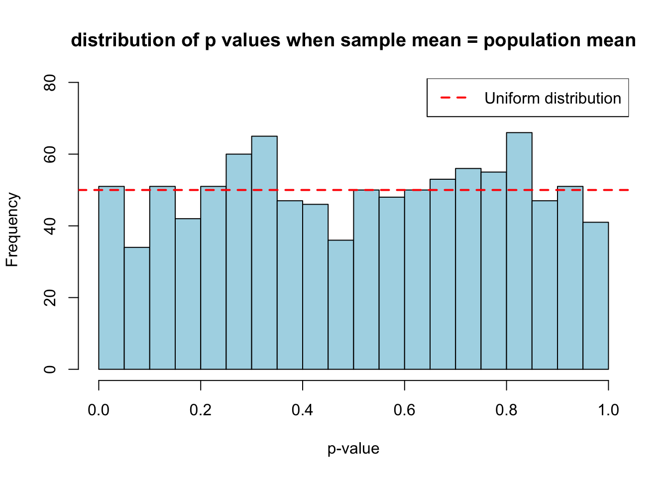

formal test against uniform distribution

qqplot(qunif(ppoints(n_simulations)), sample_pop_same,
       xlab = "Theoretical Uniform", ylab = "Observed P-values")
abline(0, 1, col = "red", lwd = 2)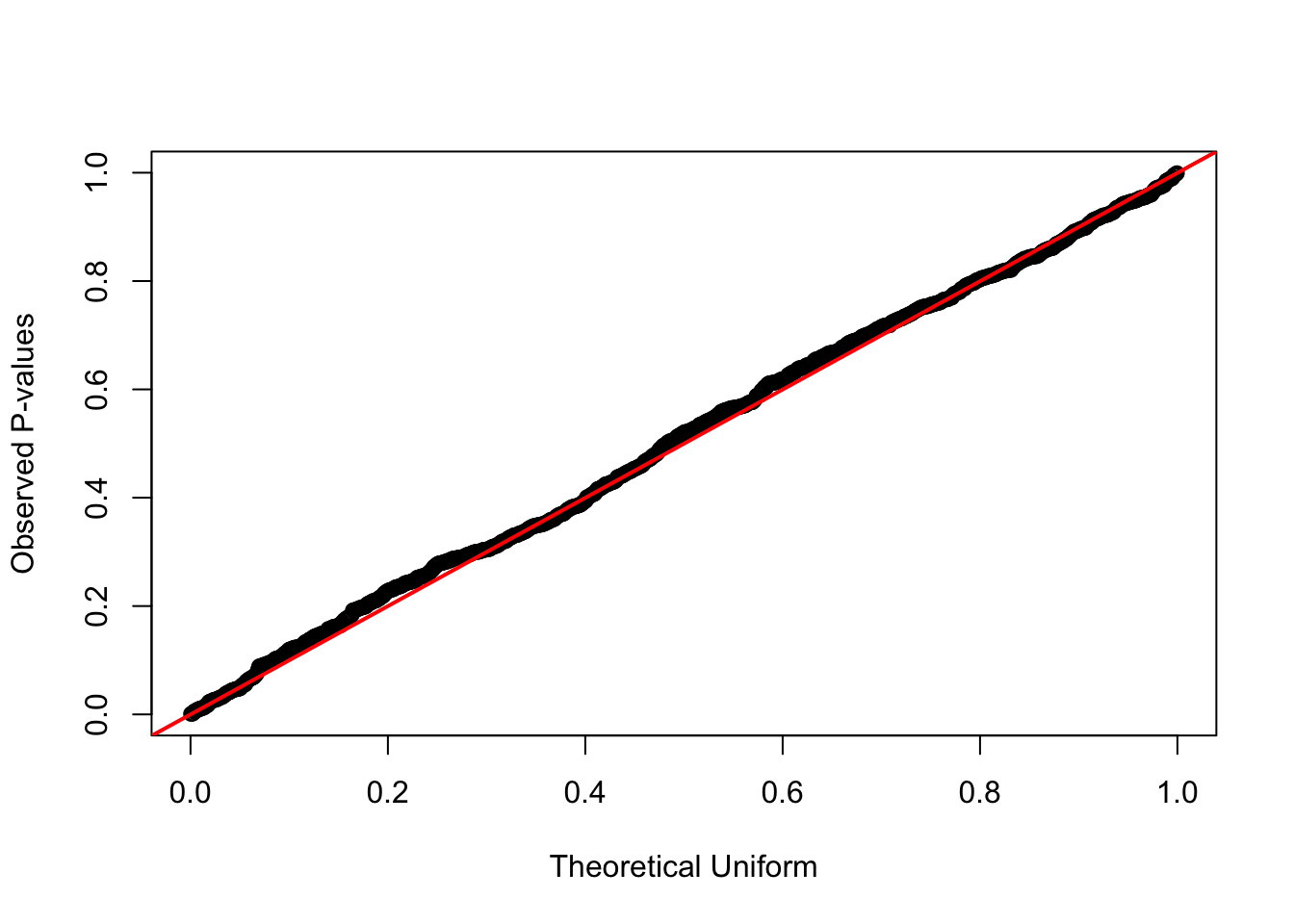

Scenario 2: sample mean is NOT the same as population mean

# create a starting point for our loop
sample_pop_diff <- numeric(n_simulations)

# create a loop to replace the values with the p-values
for (i in 1:n_simulations) {
  # Draw a sample using the population parameters
  sample_data <- rnorm(sample_size, mean = true_mean, sd = true_sd)
  
  # Test if mean = 110 (which it is not!)
  test_result <- t.test(sample_data, mu = 110)
  sample_pop_diff[i] <- test_result$p.value
}

visualise

hist(sample_pop_diff, breaks = 20, col = "lightblue", 
     main = "distribution of p values when sample mean != population mean", 
     xlab = "p-value", 
     ylim = c(0, max(table(cut(sample_pop_diff, breaks = 20))) * 1.2))
abline(h = n_simulations/20, col = "red", lwd = 2, lty = 2)
legend("topright", "skewed distribution", col = "red", lty = 2, lwd = 2)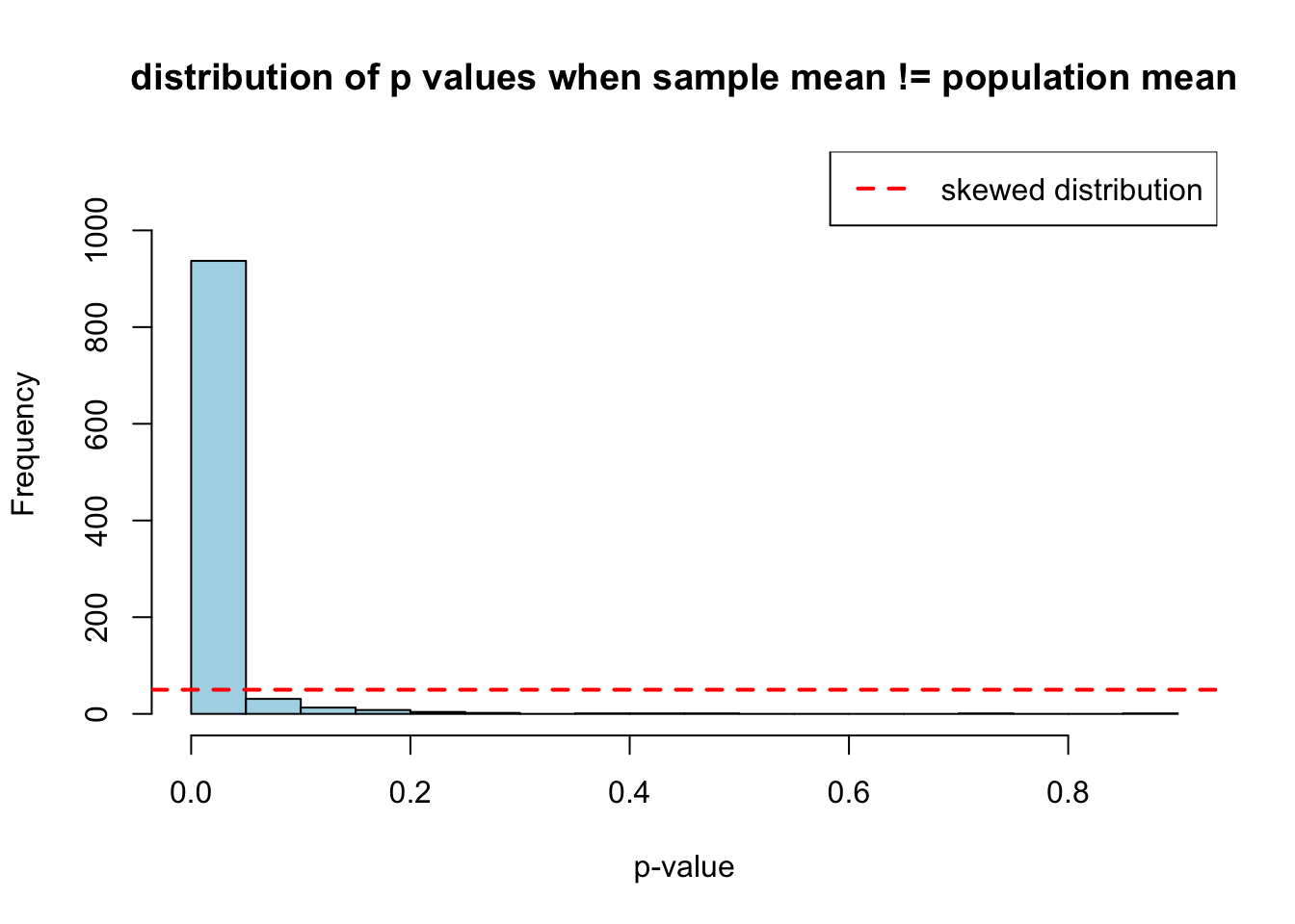

formal test against uniform distribution

qqplot(qunif(ppoints(n_simulations)), sample_pop_diff,
       xlab = "Theoretical Uniform", ylab = "Observed P-values")
abline(0, 1, col = "red", lwd = 2)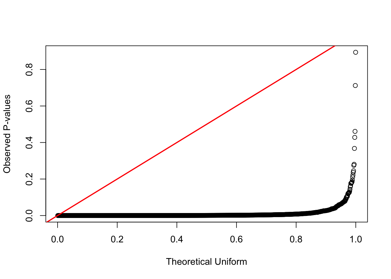

replicating a type1 error

p. 172

set.seed(42)
t.test(rnorm(10), rnorm(10))

    Welch Two Sample t-test

data:  rnorm(10) and rnorm(10)
t = 1.2268, df = 13.421, p-value = 0.241
alternative hypothesis: true difference in means is not equal to 0
95 percent confidence interval:
 -0.5369389  1.9584459
sample estimates:
 mean of x  mean of y 
 0.5472968 -0.1634567 

t.test(rnorm(10), rnorm(10))

    Welch Two Sample t-test

data:  rnorm(10) and rnorm(10)
t = 0.36582, df = 17.977, p-value = 0.7188
alternative hypothesis: true difference in means is not equal to 0
95 percent confidence interval:
 -0.8814711  1.2531201
sample estimates:
 mean of x  mean of y 
-0.1780795 -0.3639041 

t.test(rnorm(10), rnorm(10))

    Welch Two Sample t-test

data:  rnorm(10) and rnorm(10)
t = -0.082117, df = 16.257, p-value = 0.9356
alternative hypothesis: true difference in means is not equal to 0
95 percent confidence interval:
 -1.0340503  0.9568318
sample estimates:
  mean of x   mean of y 
-0.02021535  0.01839391 

t.test(rnorm(10), rnorm(10))

    Welch Two Sample t-test

data:  rnorm(10) and rnorm(10)
t = 2.3062, df = 17.808, p-value = 0.03335
alternative hypothesis: true difference in means is not equal to 0
95 percent confidence interval:
 0.06683172 1.44707262
sample estimates:
 mean of x  mean of y 
 0.5390768 -0.2178754 

“If you accept the conventional significance threshold, you expect to obtain a Type I error 5% of the time (1 in 20). Now you realize that setting the alpha level to α = 0.05 is the same as specifying how willing one is to obtain a Type I error. It’s possible to set the alpha level to a lower level, such as α = 0.01. In this case, Type I errors are expected to occur 1% of the time.” p. 173