── Attaching core tidyverse packages ──────────────────────── tidyverse 2.0.0 ──
✔ dplyr     1.1.4     ✔ readr     2.1.5
✔ forcats   1.0.1     ✔ stringr   1.5.2
✔ ggplot2   4.0.0     ✔ tibble    3.3.0
✔ lubridate 1.9.4     ✔ tidyr     1.3.1
✔ purrr     1.1.0
── Conflicts ────────────────────────────────────────── tidyverse_conflicts() ──
✖ dplyr::filter() masks stats::filter()
✖ dplyr::lag()    masks stats::lag()
ℹ Use the conflicted package (<http://conflicted.r-lib.org/>) to force all conflicts to become errors
library(palmerpenguins)
Attaching package: 'palmerpenguins'

The following objects are masked from 'package:datasets':

    penguins, penguins_raw
library(emmeans)
Welcome to emmeans.
Caution: You lose important information if you filter this package's results.
See '? untidy'
data(penguins)penguins <-drop_na(penguins)
What better way to ring in the new year than by looking at a completely different \(y\) variable related to penguins? That’s right, today we are going to take a closer look at the left side of the regression equation to talk about what happens when our outcome variable is not a number.
Specifically, we are going to look at how to model our outcome variable when it is a binary outcome: yes/no, true/false, correct/incorrect, or, in the case of our penguins, male/female.
This type of regression is called a logistic regression.
Yikes…while the right-hand side of the formula looks the same as the other regression syntax, the left-hand side is quite different. But we can understand this by thinking about something we probably already know about: the odds of something happening.
\(P\) is the probability of something
so \(P\)(\(Y\) = 1) means the probability of our outcome variable being 1 (versus 0)
Dividing the probability of something being 1 over the inverse gives us the odds of the outcome.
\[
\Large\frac{P(Y=1)}{1 - P(Y=1)}
\]
For example, assume you had a population of penguins where 80% were male and 20% were female. Let’s code female as 0 and male as 1.
The probability of being a male penguin would be 80% or .8. The odds would then be:
\[
\large\frac{0.8}{1-0.8}
\]
Which gives us the answer of \(4\) - there is \(4:1\)odds that any one penguin will be male compared to female, or four times more likely.
0.8/(1-0.8)
[1] 4
What if exactly half of the penguins were male and half were female? The odds would be \(1:1\) - equal chance:
0.5/ (1-0.5)
[1] 1
And if only .1% were male? Almost \(0:1\) odds…
0.01/ (1-0.01)
[1] 0.01010101
what happens with odds in a linear regression?
So what would happen if we fit this as a continuous variable? We would have a \(Y\) variable that goes from \(0\) to \(\infty\). The predictions would be trying to show how a one-unit increase in an \(X\) are associated with some sort of increase in the odds. This is not really a continuous variable like body mass or flipper length.
the \(ln\) function
We need a way to convert the odds into a more reasonable measure so that we can apply the regression formula. This is what the \(ln\) around the odds is - it stands for the natural logarithm. Without going into too much detail, we can think about the natural logarithm as the inversion of exponential growth in a number.
Because odds can grow to infinity, we need to bound that number into a more realistic number line. The nice thing about logged odds is that we can easily convert between the inverted logarithm and exponentiation.
# natural log of 4log(4)
[1] 1.386294
# exponent of the log of 4exp(log(4))
[1] 4
Look at what happens to this range of very different values when we apply the natural logarithm:
some_numbers =c(0.00001,1,5,10,4000,9e10)for(number in some_numbers){print(str_glue('Original value: {number} \t Natural logarithm of value: {round(log(number),3)}'))}
Original value: 1e-05        Natural logarithm of value: -11.513
Original value: 1        Natural logarithm of value: 0
Original value: 5        Natural logarithm of value: 1.609
Original value: 10       Natural logarithm of value: 2.303
Original value: 4000         Natural logarithm of value: 8.294
Original value: 9e+10        Natural logarithm of value: 25.223
natural log of odds ratio = the logit
So, now we know that the logit of the probability of a \(Y\) being 1 is the natural logarithm of the odds ratio - our dependent variable in the regression is transformed into a logit in order to describe the effects of \(x\) on \(y\).
A logistic regression is very similar to a continuous, we just need to use glm instead of lm. The glm stands for generalised linear model, a confusing term indeed, but basically lets us fit different families of distributions and different “link” functions which tells the regression how to “deal” with the distribution of the dependent variable.
For a logistic regression, we use family = binomial to tell the model that our outcome is a categorical binary variable. We then use link = logit to tell the model we want to transform the outcome variable into logits - a logistic regression.
Otherwise, the syntax is the same as lm.
glm(dv ~ x1 + x2.., family = binomial(link = 'logit'), data = dat)
inspect distribution of penguins
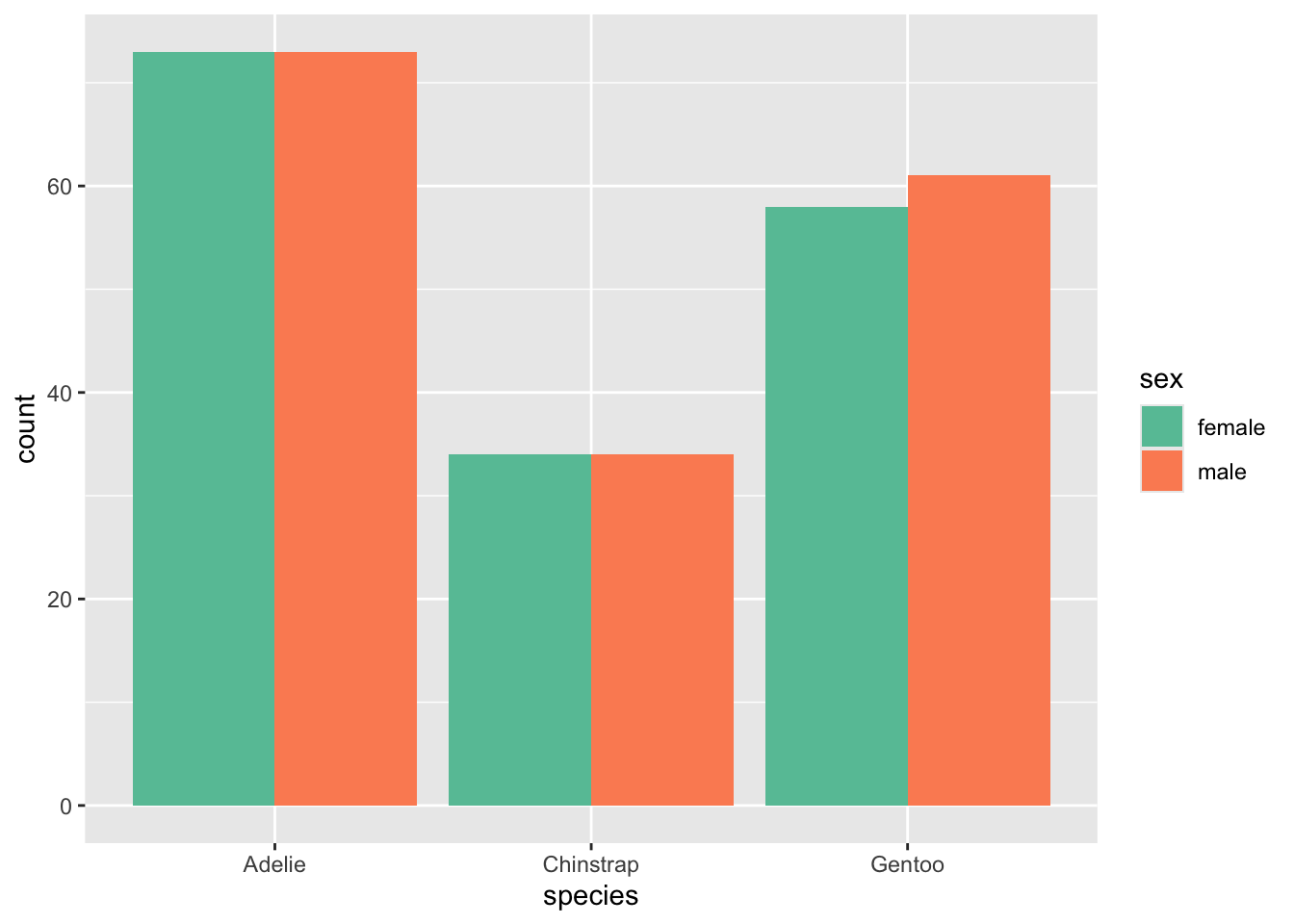
We can see that the data has a relatively balanced set of penguins, with almost exactly 50:50 ratio of male to female in the data set. So we see that species is probably not a predictor of penguin sex.
# plot the gender distributions of penguinspenguin_plot <- penguins %>%group_by(species, sex) %>%summarise(count =n())
`summarise()` has grouped output by 'species'. You can override using the
`.groups` argument.
ggplot(penguin_plot, aes(y = count, x = species, fill = sex)) +geom_col(position ='dodge') +scale_fill_brewer(palette ='Set2')
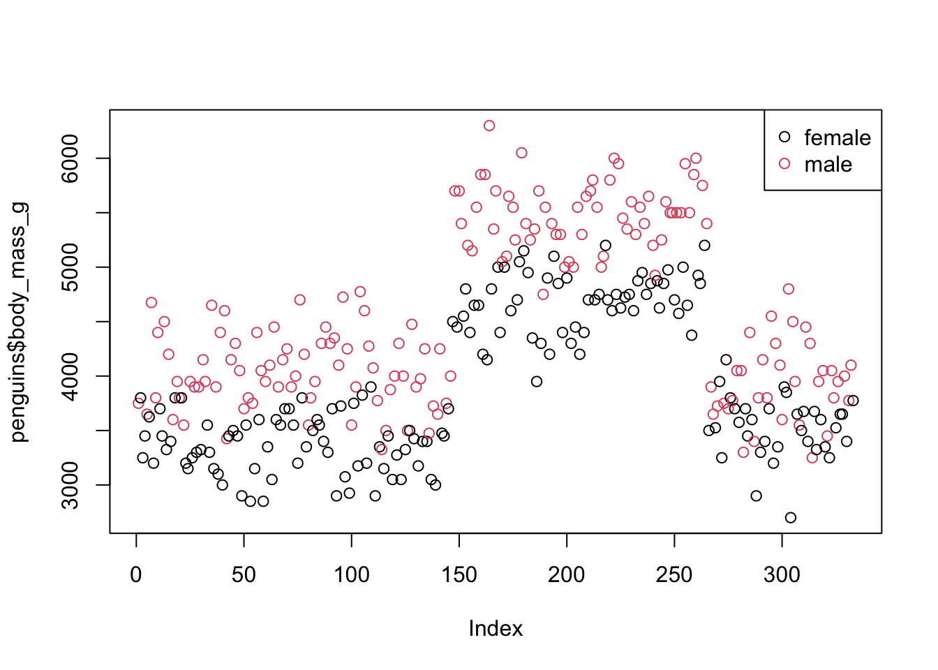
We also know that body mass is higher for male vs. female penguins
plot(penguins$body_mass_g, col = penguins$sex)legend('topright', legend =levels(penguins$sex), col =1:2, pch =1)
predict sex with body mass
Lets flip predict penguin sex with body mass. Let’s z-score body mass
Here is the simple one predictor regression model:
# fit a logistic regression predicting sex from body mass:m1 <-glm(sex ~ body_mass_z, family =binomial(link ='logit'), data = penguins)summary(m1)
Call:
glm(formula = sex ~ body_mass_z, family = binomial(link = "logit"),
    data = penguins)

Coefficients:
            Estimate Std. Error z value Pr(>|z|)
(Intercept)  0.05345    0.12184   0.439    0.661
body_mass_z  0.99832    0.13909   7.177  7.1e-13 ***
---
Signif. codes:  0 '***' 0.001 '**' 0.01 '*' 0.05 '.' 0.1 ' ' 1

(Dispersion parameter for binomial family taken to be 1)

    Null deviance: 461.61  on 332  degrees of freedom
Residual deviance: 396.64  on 331  degrees of freedom
AIC: 400.64

Number of Fisher Scoring iterations: 4
How do we interpret this? We do so in the same way as the lm regressions. The intercept is the predicted logit value of our outcome variable, and the estimates are the effects of the predictor variable. However, now that our outcome variable is expressed in terms of logits, it becomes more difficult to make any sense of these estimates.
Note
Recall that the logit is the log of the log odds.
Here the intercept is close to 0, which is similar to an odds ratio of 1:1, which represents a 50% probability of either category (even odds).
Refer to Table 12.1 on p. 203 of Winter (2019)
Female penguins are the baseline, coded as 0, whereas male penguins are coded as 1. So positive effects indicate a movement towards 1 (in this case, a movement towards male). The intercept of 0.053 represents the predicted logit when body mass is at the mean (i.e., when body_mass_z = 0), which corresponds to roughly even odds of being male or female penguin.
what about the coefficient?
The estimate for body_mass_z is 0.998, meaning that a one standard deviation increase in body mass is associated with an increase of 0.998 logits. Because this value is close to 1 on the logit scale, it represents a fairly substantial shift in the predicted probability of being male as body mass increases by one standard deviation.
back transforming the logit
We can convert the logit back to an odds scale, because the logarithm can be inversed using exponentiation. The estimate for the effect of body mass increase was 0.998, so the odds ratio would be:
exp(0.998)
[1] 2.712851
This gives an odds ratio of 2.71, meaning that a one standard deviation increase in body mass is associated with 2.71:1 odds of being male compared to female.
Converting the ratio to a percentage means subtracting 1 from the value and then multiplying by 100 - here we get 171 or 171%
(2.71-1) *100
[1] 171
So an increase in one standard deviation of body mass is associated with a 171% increase in the odds that a penguin will be male compared to female.
using emmeans
the emmeans package lets us swap between these as well. Note the message given here - that the results are on the logit scale, NOT the response scale. You should understand what this means now - the response scale is the original scale, which is expressed as frequency tallies or percentages. The logits were formed as part of the model building process.
emmeans(m1, ~ body_mass_z)
 body_mass_z emmean    SE  df asymp.LCL asymp.UCL
   -1.37e-16 0.0534 0.122 Inf    -0.185     0.292

Results are given on the logit (not the response) scale.
Confidence level used: 0.95
We can ask for the results to be expressed on the original scale, which is expressed a probability. How to interpret this output? When body_mass_z is held at the mean, 0, there is a 51.3% chance that the penguin is a male penguin. That’s almost even odds (e.g., odds ratio of 1).
emmeans(m1, ~ body_mass_z, type ='response')
 body_mass_z  prob     SE  df asymp.LCL asymp.UCL
   -1.37e-16 0.513 0.0304 Inf     0.454     0.573

Confidence level used: 0.95
Intervals are back-transformed from the logit scale
Using emtrends, we get the statistical effect (or slope, trend, whatever) of body mass on sex, which is the 0.998 logits discussed earlier.
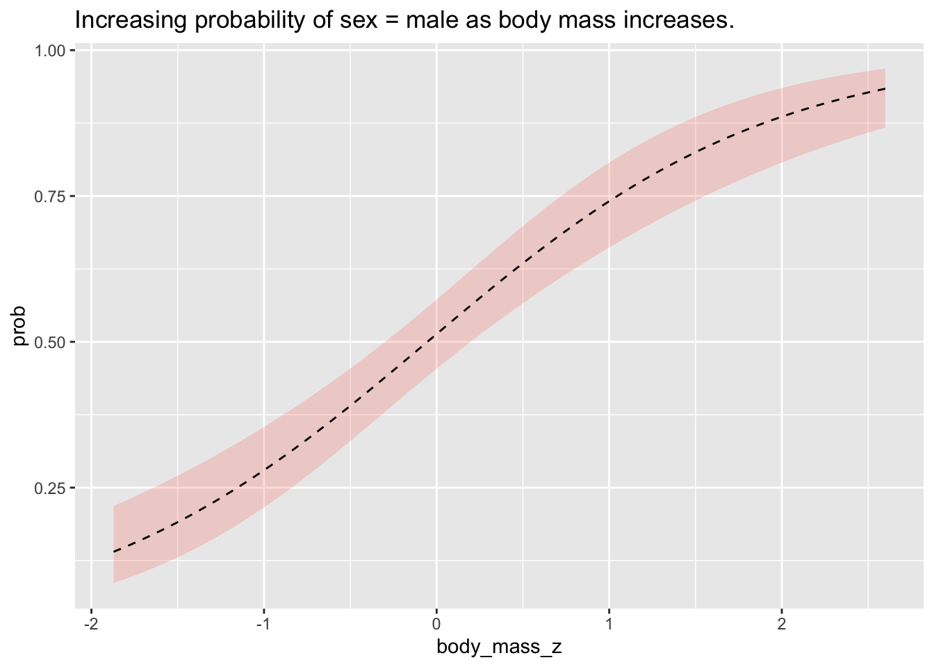
We can plot the probabilities at different emmeans to show the probability contours, which is an incredibly intuitive way to visualise the effects of a logistic regression.
Because the level female in the variable sex was the baseline, coded as 0, the model is trying to predict the probability of male, which was coded as 1. Here, they y-axis is the percentage likelihood the outcome variable will be 1 (i.e., sex == male).
prob_plot <-as.data.frame(emmeans(m1, ~body_mass_z, type ='response', at =list(body_mass_z =seq(min(penguins$body_mass_z), max(penguins$body_mass_z), length.out =100))))ggplot(prob_plot,(aes(y = prob, x = body_mass_z))) +geom_ribbon(aes(ymin = asymp.LCL, ymax = asymp.UCL), alpha = .25, fill ='salmon') +geom_line(lty ='dashed') +labs(title ="Increasing probability of sex = male as body mass increases.")
Once you understand how a logistic regression can be interpreted, it becomes no different than the linear regressions we’ve been looking at before. The tricky bit is usually making sure we understand the difference between logits (also called log odds), odds ratios, and probabilities.